22.3.1.1. Simulink Host Mode
For the synchronous simulation of control design tool and RecurDyn, following four steps are required as shown in Figure 22.21.
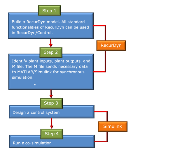
Figure 22.21 Four-step process
Communication sequence
Make the shared memory and RecurDyn is called by Simulink, wait the Plant output (2) of RecurDyn.
Send plant outputs and wait control outputs (4) of the Simulink.
Receive sensor inputs (=plant output) from the shared memory.
Send control outputs from Simulink.
Receive plant inputs (=control output) from shared memory.

Figure 22.22 Communication Sequence
22.3.1.1.1. Step I (In RecurDyn)
Step to open the RecurDyn model
The model is provided in the RecurDyn installation directory <Install Dir>\Help\Examples\Simulink_CoSim\.
Create a new working directory.
Copy the RecurDyn model(mouse.rdyn) and Simulink model(simouse.mdl) from the directory paste to the newly created working directory.
Run RecurDyn.
Open the RecurDyn model. And then, the mouse model appears in the working window.
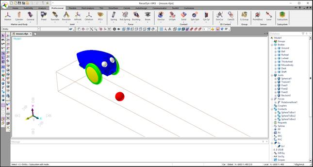
Figure 22.23 Mouse model
Step to verify the mechanical system model
Prior to applying a control system to this model, make sure that the mouse model runs without any errors.
Select Dynamic/Kinematic icon of the Simulation group in the Analysis tab.
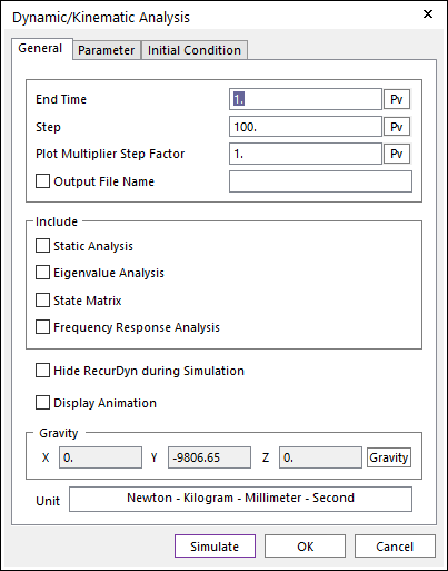
Figure 22.24 Dynamic/Kinematic Analysis dialog box
Enter End time and Step.
Click Simulate.
If the simulation stops abnormally, fix the model and try the simulation again.
22.3.1.1.2. Step II (In RecurDyn)
Step to identify general GPlant inputs
The input of interest is the single rotational axial force is applied to the wheel Revolute Joint to move the mouse.
Click the GPlant_Input icon of the Control group in the Communicator tab. The General GPlant Input List dialog box appears as shown in Figure 22.25. For more information, click here.
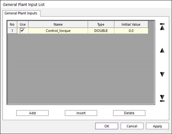
Figure 22.25 General GPlant Input List dialog box
Add a GPlant input as the name of the actuator.
Add an expression function as a following figure.
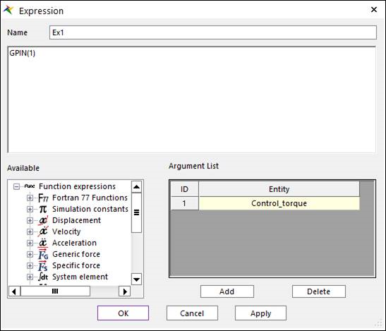
Figure 22.26 Expression dialog box
Open the dialog box of Rotational Axial force by double clicking RotationalAxial1 in the Database window. And then input the expression function defined in the upper step.
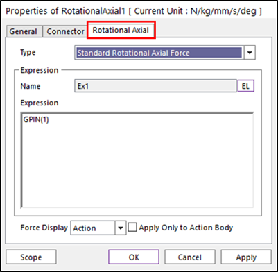
Figure 22.27 Rotational Axial force dialog box
Step to identify general GPlant outputs
The output of interest is the displacement and velocity between the ball and the Mouse body pointer. This distance is in the X direction.
Click the. GPlant_Output icon of the Control group in the Communicator tab. The General Plant Output List dialog box appears as shown in Figure 22.28. For more information, click here.
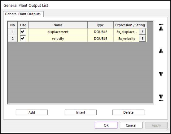
Figure 22.28 General Plant Output dialog box
Add GPlant outputs as expression functions. At this dialog, the defined expression functions are as following figures.

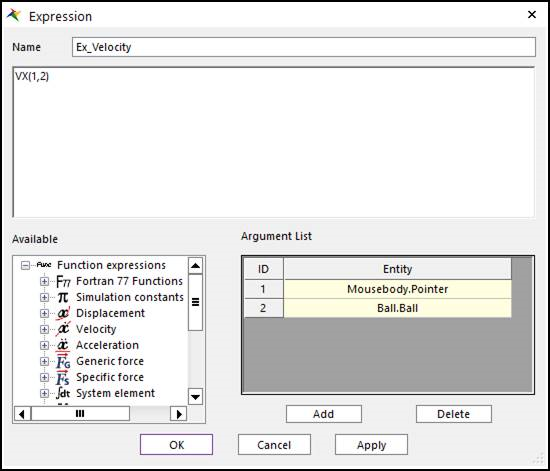
Figure 22.29 Expression dialog box
Step to set interface information
Save the RecurDyn model in the normal fashion.
Click the GCoSim icon of the Control group in the Communicator tab. The General CoSim dialog box appears. For more information, click here.
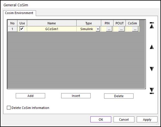
Figure 22.30 General CoSim dialog box
Click Add button.
Define the name of General CoSim as “GCoSim1”.
Select the type of General CoSim as Simulink.
Click the PIN (…) button. The General GPlant Input List (GCoSim1) dialog box appears.
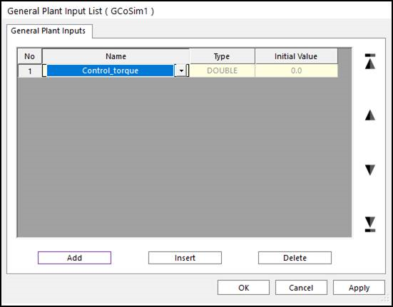
Figure 22.31 General GPlant Input List (GCoSim1) dialog box
Click Add button. Automatically “Control_torque” is input. And click OK button.
Likewise Clink the POUT (…) button. The General GPlant Output List (GCoSim1) dialog box appears.
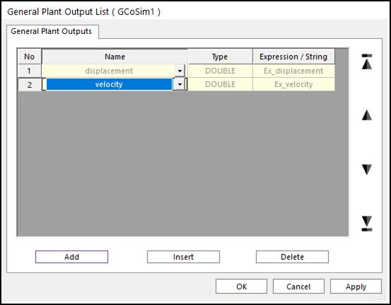
Figure 22.32 General GPlant Output List (GCoSim1) dialog box
Click Add button twice. Automatically “displacement” and “velocity” are input. And Click OK button.
Click CoSim(…) button. The Simulink (GCoSim1) dialog box appears.
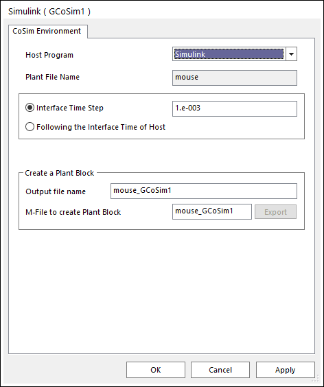
Figure 22.33 Simulink (GCoSim1) dialog box
Select the Host Program as Simulink.
Export the M file to create a Plant Block after defining the names.
Edit Sampling Period (Control Time Step).
Check Use Identical Solution of RDHost Option.
Click OK.
Save the RecurDyn model and terminate the RecurDyn program.
22.3.1.1.3. Step III (In MATLAB)
Step to build Simulink model with RecurDyn Plant Block
Run the MATLAB program.
Change the working directory to the directory that includes the M file and RecurDyn model.
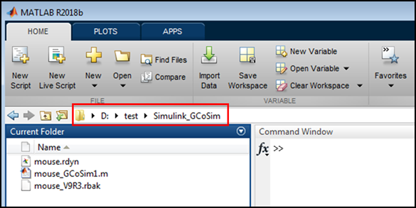
Figure 22.34 Changing the working directory
In the MATLAB command window, enter the name of M file.
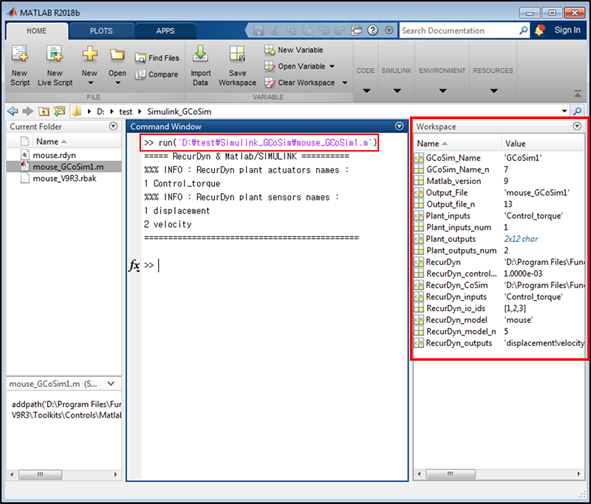
Figure 22.35 Reserved variables from M file
In the MATLAB command window, enter GRDClient.
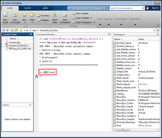
Figure 22.36 Entered GRDClient
And then, a new Simulink window with RecurDyn Plant Block appears.
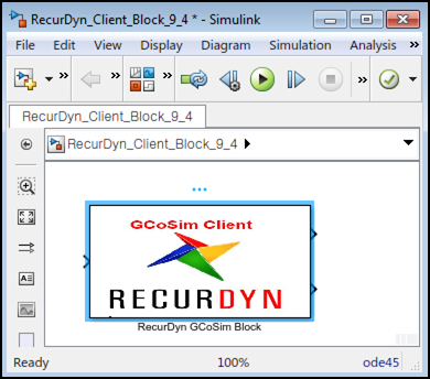
Figure 22.37 RecurDyn Plant Block
Open the Simulink model (simouse.mdl).
Drag and drop RecurDyn Plant Block on the opened Simulink model window.
Construct the control algorithm as shown in Figure 22.38.
Save the Simulink model.
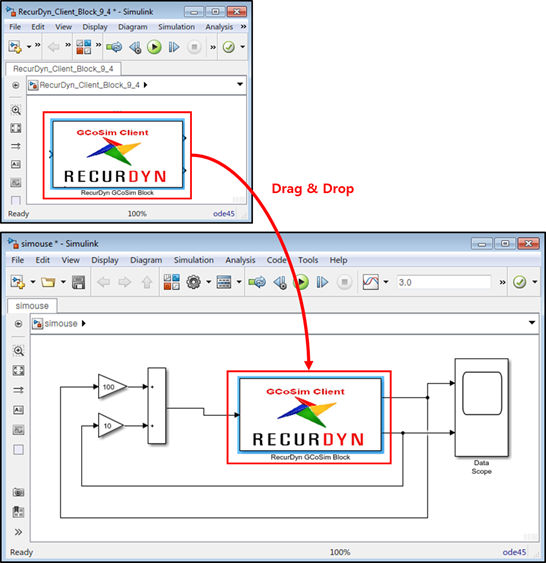
Figure 22.38 Steps to design control algorithm
22.3.1.1.4. Step IV (In MATLAB)
Step to do the co-simulation
Double-click the RecurDyn Plant Block. The sub block of the RecurDyn Plant Block appears.
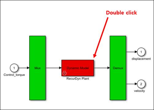
Figure 22.39 Steps to design control algorithm
Double-clicks the Red block (Dynamic Model). The Block Parameters dialog box appears.
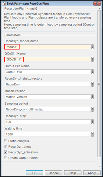
Figure 22.40 Function Block Parameters dialog box
Change RecurDyn_model_name as ‘mouse’.
Change GCoSim Name as ‘GCoSim1’.
Click OK.
Select Configuration Parameters in the Simulink menu.
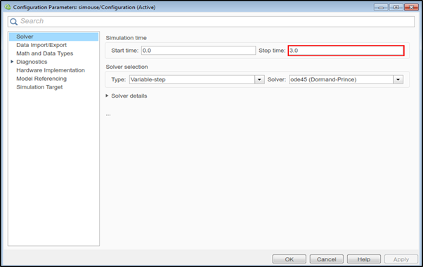
Figure 22.41 Steps to run co-simulation
Change the Stop time to 3.0 seconds.
Click OK
Click Start in the Simulation menu.
22.3.1.1.5. Step V (In RecurDyn)
Step to see the Animation Result
In RecurDyn, play the animation.
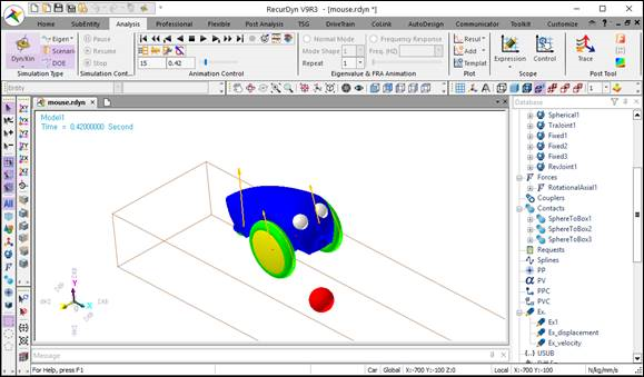
Figure 22.42 Show the animation
Step to see the Plot Result
To plot the output data, click the Result icon of Plot group in Analysis tab.
Expand the Plant Input item in the database window on the right side. Expand the Control_torque. Double-click on Value in the section and adjust the label and axes to get the plot below.
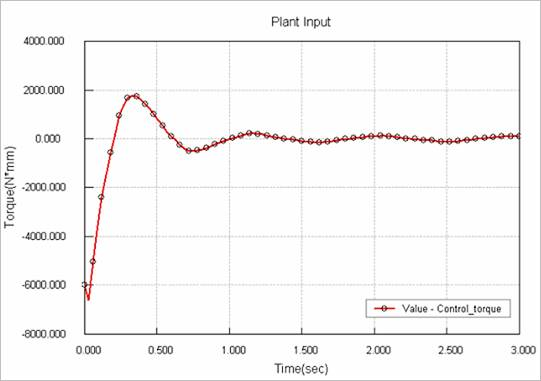
Figure 22.43 Plot of Value - Control_torque
Expand the Plant Output item. Expand the displacement and velocity and double-click on each Value.
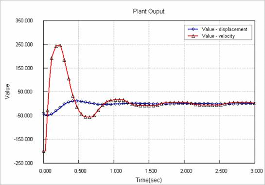
Figure 22.44 Plot of Value - displacement and Value-velocity