39.1.2.2. Additional Options
The user can control the viscosity information and the asperity contact information.
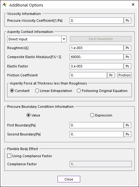
Figure 39.12 Additional Options dialog box
Pressure-Viscosity Coefficient [1/Pa]: The user can use the dynamic viscosity as the function of pressure as shown in a following equation. When the pressure-viscosity coefficient is not zero, the defined dynamic viscosity work as the value measured in the atmosphere pressure, \({{\mu }_{0}}\,\). If relative large pressure-viscosity coefficient is input, numerical solution can be diverged because it is the exponent of exponential function. So, appropriate value should be selected. There are some examples of pressure-viscosity coefficient for various fluids in figure 2.
\(\mu ={{\mu }_{0}}{{e}^{\alpha p}}\)
- Where,
- \(\alpha\) is the viscous-pressure coefficient[\(1/ P_a\)]\(\mu\) is the dynamic viscosity and it is a function of pressure[\(Pa \cdot s\)]\({\mu }_{0}\) is the dynamic viscosity measured in the atmosphere pressure [\(Pa \cdot s\)]
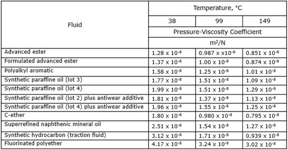
Figure 39.13 Examples of Pressure-Viscosity Coefficient [From Jones et al. (1975)]
Asperity Contact Model: In the case of mixed lubrication region, the asperity contact force is added into the fluid pressure. The equation for asperity contact model is as follows:
\(\begin{aligned} & {{P}_{a}}(h)=K{{E}^{'}}{{F}_{5/2}}\left( h/{{\sigma }_{s}} \right) \\ & {{F}_{5/2}}\left( h/{{\sigma }_{s}} \right)=4.4086\times {{10}^{-5}}{{\left( 4-h/{{\sigma }_{s}} \right)}^{6.804}} \\ \end{aligned}\)
- Where,
- \({P}_{a}\) is the asperity contact pressure [\(F/{{L}^{2}}\)].\(h\) is the ilm thickness [\(L`\)].\({\sigma}_{s}\) is the composite roughness [\(L\)].\(K\) is the elastic factor.\({E}^{'}\) is the composite elastic modulus [\(F/{{L}^{2}}\)].
Asperity Force at Thickness less than Roughness: In the case that clearance (gap between two bodies in contact) is lower than roughness, asperity contact force becomes larger too much according to equation of asperity contact model. Special treat for asperity contact model is evaluated in this case.
Constant: In this type, if clearance is lower than the roughness, asperity contact pressure is always same as asperity contact pressure at the situation that clearance is same as roughness.
Linear Extrapolation: In this type, if clearance is lower than the roughness, asperity contact force is extrapolated with the tangent of equation of asperity contact model at the situation that clearance is same as roughness.
Following Original Equation: In this type, calculation of asperity contact force just follows the equation of asperity contact model regardless of size of clearance.
Direct Input: Define asperity contact information such as composite roughness, composite elastic modulus and elastic factor.
Each Parameter & Calculation: Define property of each action and base body such as elastic modulus, poisson’s ratio, roughness, number of asperities per unit area, mean radius of curvature of the asperities respectively. And then, calculate composite asperity property using this data.
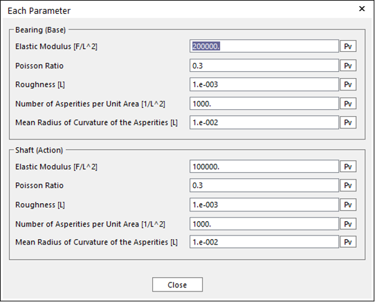
Figure 39.14 Each Parameter Setting in Asperity Contact Information
Composite roughness, elastic modulus and elastic factor can be computed using each surface property of action and base body. The relationship formula is as follows.
\(\begin{aligned} & {{\sigma }_{s}}=\sqrt{{{\sigma }_{a}}^{2}+{{\sigma }_{b}}^{2}} \\ & {{E}^{'}}=\frac{1}{\left( \frac{1-{{\nu }_{a}}^{2}}{{{E}_{a}}} \right)+\left( \frac{1-{{\nu }_{b}}^{2}}{{{E}_{b}}} \right)} \\ & K=\frac{16\sqrt{2}}{15}\pi {{\left( {{\sigma }_{s}}\beta \eta \right)}^{2}}\sqrt{\frac{{{\sigma }_{s}}}{\beta }} \\ & \eta =\sqrt{{{\eta }_{a}}{{\eta }_{b}}}\,\,\,,\,\,\,\,\beta ={{\left( \frac{1}{2{{\beta }_{a}}}+\frac{1}{2{{\beta }_{b}}} \right)}^{-1}} \\ \end{aligned}\)
- Where,
- \({\sigma }_{a}\), \({{\sigma }_{b}}\) : roughness of each body.\({{\eta }_{a}}\), \({{\eta }_{b}}\) : asperity number of unit area.\({{\beta }_{a}}\), \({{\beta }_{b}}\) : meanradius of curvature of the asperities.
Pressure Boundary Condition [Pa]: First Boundary means the boundary pressure at the end of the negative z direction of base marker and Second Boundary means the boundary pressure at the end of the positive z direction of base marker. User can input boundary pressure for both end position in axial direction through this functionality. Input unit is Pascal.
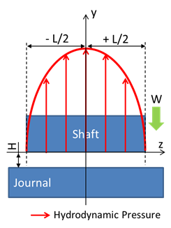
Figure 39.15 Pressure Boundary