21.3.9.5. Multiple Performance Indexes

When one evaluates the failure probability for multiple performance indexes, Monte-Carlo simulation gives failure probability for each performance respectively. SAO based hybrid method, however, gives failure probability for critical limit.

In order to help one’s understand for them, let’s solve the reliability analysis problem having two performance indexes shown in Figure 21.131. The mean point is (3,3) and their standard deviation are (1,2). Also, suppose that DV1 is ‘normal distribution’ and DV2 is Weibul distribution.

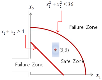
Figure 21.131 Reliability analysis problem for two performance indexes

SAO based Hybrid Method

As SAO method solves to find the nearest point from mean point to while satisfying PI=0. Thus, it can’t help solving m times optimization problems for m performance indexes. It requires many evaluations. Thus, AutoDesign finds the critical MPP that is the nearest point among MPPs form performance indexes. From the view point of design, an optimal design should satisfy all constraints simultaneously. Thus, we find only critical MPP. Figure 21.132 explains finding the critical MPP graphically.

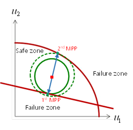
Figure 21.132 Graphical representation of critical MPPs

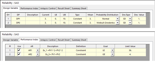
As it is just a mathematical example, we create a dummy model. Then, we can express the problem of Figure 21.131 by defining two parameters PV1 and PV2 as random variables and defining two relations composed of them as constraints as shown in the figure below.

In addition, since it is a mathematical problem, the convergence tolerance is strictly set in consideration of the absence of numerical noise. Then, the initial sample point is selected by the Koshal method. In this method, first metamodel is created with 1 + NDV points, and a new point is obtained by the HLRF method. Then take an additional number of NDVs around the new point.

Figure 21.133 shows the convergence history. AR2 is the critical performance index. AFORM gives that failure probability is 0.082052.

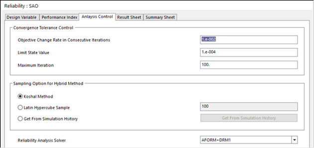
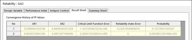
Figure 21.133 Convergence history of SAO based Hybrid method

Figure 21.134 shows Summary Sheet. As DV2 (DP2) is uniform distribution, Param_1 and Param_2, internally calculated, are shown. Next, in Performance Index (Result), AR2 is nearly ‘zero’ at MPP. This represents that AR2 is nearer than AR1 from Mean point in the normalized space.

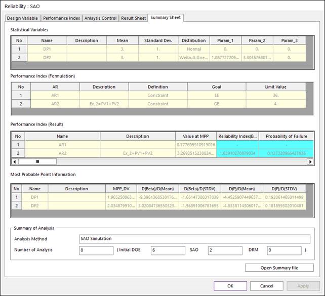
Figure 21.134 Summary of SAO based Hybrid method

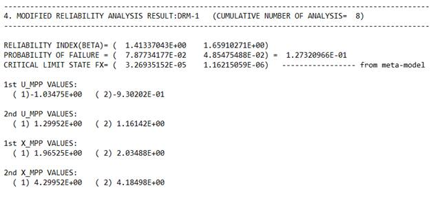
However, it should be noted that the final failure probability is ‘0.12732’. Even though DRM1 compensates for the failure probability, the difference between the values of the failure probability is too large in comparison with the convergence result in Figure 21.133. So, to see the convergence process in detail, let’s open the Summary file.

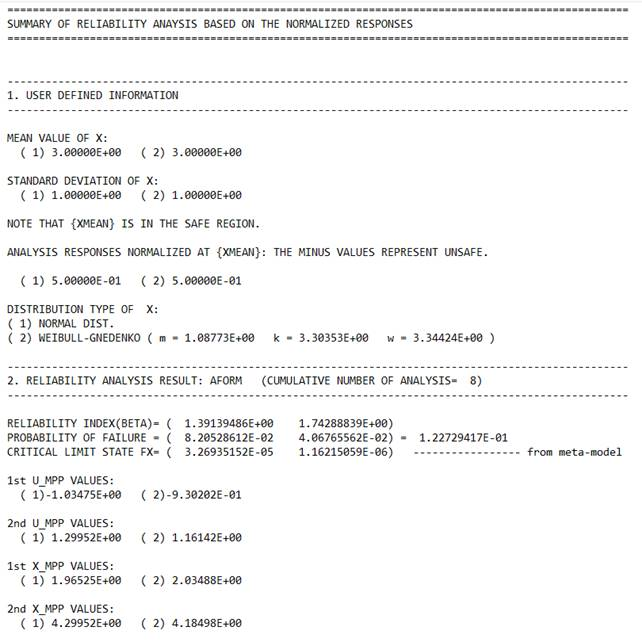
As we predicted in Figure 21.132, we can see that there are two MPPs in the above summary. Thus, the finally determined failure probability is the sum of the failure probabilities of these MPPs.

Monte-Carlo Simulation

Unlike SAO method, Monte-Carlo simulation didn’t solver optimization problem. It just samples points and evaluate performance indexes. Then, it counters the number of points in the failure zone. Thus, the parallel computation can be easily implemented. Figure 21.135 shows the summary of Monte-Carlo simulation with 100 sample points.

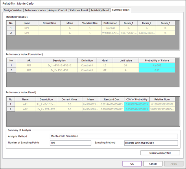
Figure 21.135 Summary of Monte-Carlo simulation

The Monte-Carlo results show that the predicted failure probability differs from the SAO method. This is because the number of sample points is insufficient to predict the failure probability. When the failure probability is 0.127, the number of suitable sample points is as follows.

\(N=396\text{ }\left( \frac{1-0.127}{0.127} \right)\approx 2272\)