4.7.1.9. Polynominal
4.7.1.9.1. BISTOP
The BISTOP function returns the contact force of a model in a gap defined by the relative location and velocity of two markers.
Format
Arguments definition
Distance(\(x\)) |
The relative distance between the two markers on the contacting entities |
Velocity(\(\dot{x}\)) |
The relative velocity between the two markers on the contacting entities |
Free length1(\({{x}_{1}}\)) |
The contact distance between the two markers on the contacting entities - This value must be a real number or a function that returns a real number. - The free length(x1) is used to determine whether or not contact is made. |
Free length2(\({{x}_{2}}\)) |
The contact distance between the two markers on the contacting entities - This value must be a real number or a function that returns a real number. - Free length(x2) is used to determine whether or not contact is made. |
Stiffness(\(k\)) |
The modulus rigidity on the spring force |
Stiffness exponent(\(\exp\)) |
The nonlinear coefficient value on the surface of the spring force |
Damping(\({{c}_{\max }}\)) |
The maximum damping coefficient This must be a real number or a function that returns a real number |
Penetration(\(d\)) |
The depth of infiltration that induces the maximum damping coefficient |
(Bistop= 0, When Bistop<0) and (“Bistop= 0, When Bistop>0 )
: It is the same meaning that Rebound Damping Factor is ZERO.
Formulation
\(\text{BISTOP =}\left\{ \begin{aligned} & k{{({{x}_{1}}-x)}^{\exp }}-\text{STEP}(x,{{x}_{1}}-d,{{c}_{\max }},{{x}_{1}},0)\cdot \dot{x}\,\,\,\,\text{when},\text{ }x<\,{{x}_{1}} \\ & 0\,\,\,\,\,\,\,\,\,\,\,\,\,\,\,\,\,\,\,\,\,\,\,\,\,\,\,\,\,\,\,\,\,\,\,\,\,\,\,\,\,\,\,\,\,\,\,\,\,\,\,\,\,\,\,\,\,\,\,\,\,\,\,\,\,\,\,\,\,\,\,\,\,\,\,\,\,\,\,\,\,\,\,\,\,\,\,\,\,\text{when},x<\,{{x}_{1}}\And \text{BISTOP}<0) \\ & 0\,\,\,\,\,\,\,\,\,\,\,\,\,\,\,\,\,\,\,\,\,\,\,\,\,\,\,\,\,\,\,\,\,\,\,\,\,\,\,\,\,\,\,\,\,\,\,\,\,\,\,\,\,\,\,\,\,\,\,\,\,\,\,\,\,\,\,\,\,\,\,\,\,\,\,\,\,\,\,\,\,\,\,\,\,\,\,\,\,\text{when},\text{ }{{x}_{1}}\le x<{{x}_{2}}, \\ & -k{{(x-{{x}_{2}})}^{\exp }}-\text{STEP}(x,{{x}_{2}},0,{{x}_{2}}+d,{{c}_{\max }})\cdot \dot{x}\,\,\,\text{when},\text{ }x\ge {{x}_{2}} \\ & 0\,\,\,\,\,\,\,\,\,\,\,\,\,\,\,\,\,\,\,\,\,\,\,\,\,\,\,\,\,\,\,\,\,\,\,\,\,\,\,\,\,\,\,\,\,\,\,\,\,\,\,\,\,\,\,\,\,\,\,\,\,\,\,\,\,\,\,\,\,\,\,\,\,\,\,\,\,\,\,\,\,\,\,\,\,\,\,\,\,\,\text{when},x\ge {{x}_{2}}\And \text{BISTOP}>0) \\ \end{aligned} \right.\)
Example
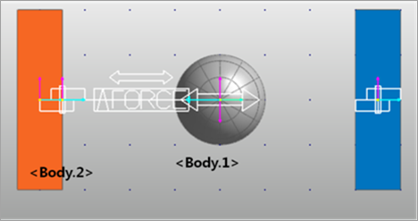
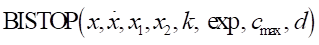
Figure 4.55 Example modeling for the BISTOP function
BISTOP(DX(Body1.Marker2,Body2.Marker1,Body2.Marker1),VX(Body1.Marker2,Body2.Marker1,Body2.Marker1),150,600,10000,1.3,100,2)
\({x}\) = DX: Distance variable
\(\dot{x}\) = VX: Time derivative of x
\({x}_{1}\) = 150: Lower bound of x
\({x}_{2}\) = 600: Upper bound of x
\({k}\) = 10000: Stiffness
\({exp}\) = 1.3: Exponent of force
\({c}_{\max}\) = 100: Maximum damping coefficient
\({d}\) = 2: Boundary penetration
Figure 4.56 Scope result using the BISTOP function
4.7.1.9.2. CHEBY
The CHEBY function returns the result of the coefficients and variables evaluated using the Chebyshev polynomial.
Format
Arguments definition
\({x}\) |
The input variable for the Chebyshev equation - Generally, this variable is a real number, function, or time. |
\({x}_{0}\) |
The x-direction offset for the variable (\(\text{x}\)) in the Chebyshev polynomial |
\({c}_{0}, {c}_{1}, \cdots, {c}_{30}\) |
The coefficient values in the Chebyshev polynomial that calculate the linear superposition in line with the Chebyshev polynomial - These values are defined by the number of input coefficients and can include up to 31 coefficients. |
Formulation
\(\begin{aligned} & \text{C(x)}=\sum\limits_{j=0}^{n}{{{c}_{j}}\cdot {{T}_{j}}(x-{{x}_{0}})\,\,\,\,\,\,\,\,\,\,\,\,0\le j\le n} \\ & \left( \begin{aligned} & \text{where,}\,\,{{T}_{j}}(x-{{x}_{0}})=2\cdot (x-{{x}_{0}})\cdot {{T}_{j-1}}(x-{{x}_{0}})-{{T}_{j-2}}(x-{{x}_{0}}) \\ & \,\,\,\,\,\,\,\,\,\,\,\,\,\,\,\,{{T}_{0}}(x-{{x}_{0}})=1,\,\,\ {{T}_{1}}(x-{{x}_{0}})=x-{{x}_{0}} \\ \end{aligned} \right) \\ \end{aligned}\)
Example
CHEBY (time, 1, 1, 1, 1)
\({x}\) = time: Independent variable
\({x}_{0}\) = 1: Shift in the Chebyshev polynomial
\({c}_{0}\), \({c}_{1}\), \({c}_{2}\): Define coefficient for the Chebyshev polynomial
\({c}_{0}\) = 1, \({c}_{1}\) = 1, \({c}_{2}\) = 1
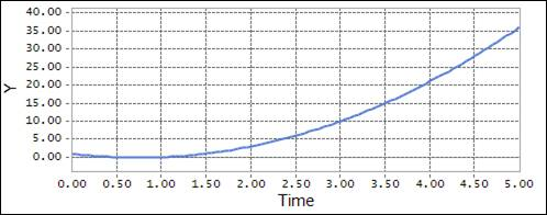
Figure 4.57 Scope result using the CHEBY function
4.7.1.9.3. FORCOS
The FORCOS function returns the results of the coefficients and variables evaluated in a Fourier Cosine series.
Format
Arguments definition
\({x}\) |
The input variable for the defined Fourier Cosine series - Generally, this variable is time or a function that results in a real number. |
\({x}_{0}\) |
The x-direction offset for the variable (x) in the Fourier Cosine series |
\({\omega}\) |
The base frequency for the Fourier Cosine series (in radians) |
\({c}_{0}, {c}_{1}, \cdots, {c}_{30}\) |
The coefficient values in the Fourier cosine series that calculates the linear superposition in line with the Fourier cosine series - These values are defined by the number of input coefficients and can include up to 31 coefficients. |
Formulation
\(\begin{aligned} & \text{F(x)=}{{c}_{0}}+\sum\limits_{j=1}^{n}{{{c}_{j}}\cdot {{T}_{j}}(x-{{x}_{0}})\,\,\,\,0\le j\le n} \\ & \left( where\,\,\,\,\,\,\,\,\,\,\,{{T}_{j}}(x-{{x}_{0}})=\cos [j*\omega *(x-{{x}_{0}})] \right) \\ \end{aligned}\)
Example
FORCOS(time, 0, 360D, 1, 2, 3)
\({x}\) = time: Independent variable
\({x}_{0}\) = 0: Shift in the Fourier cosine series
\({\omega}\) = 360D: Frequency of the Fourier cosine series
\({c}_{0}\), \({c}_{1}\), \({c}_{2}\) : Define coefficient for the Fourier series
\({c}_{0}\) = 1, \({c}_{1}\) = 2, \({c}_{2}\) = 3
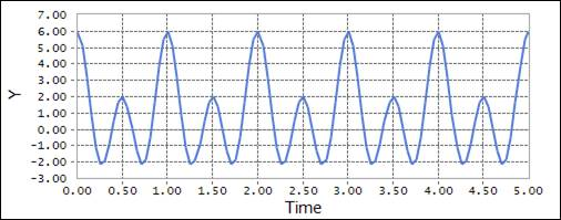
Figure 4.58 Scope result using the FORCOS function
4.7.1.9.4. FORSIN
The FORSIN function returns the results of the coefficients and variables evaluated in a Fourier sine series.
Format
Arguments definition
\({x}\) |
The input variable for the defined Fourier sine series - Generally, this variable is time or a function that results a real number. |
\({x}_{0}\) |
The x-direction offset for the variable (x) in the Fourier sine series |
\({\omega}\) |
The base frequency for the Fourier sine series (in radians) |
\({c}_{0}, {c}_{1}, \cdots, {c}_{30}\) |
The coefficient values in the Fourier cosine series that calculates the linear superposition in line with the Fourier cosine series - These values are defined by the number of input coefficients and can include up to 31 coefficients. |
Formulation
\(\begin{aligned} & \text{F(x)=}{{c}_{0}}+\sum\limits_{j=1}^{n}{{{c}_{j}}\cdot {{T}_{j}}(x-{{x}_{0}})\,\,\,\,0\le j\le n} \\ & \left( where\,\,\,\,\,\,\,\,\,\,\,{{T}_{j}}(x-{{x}_{0}})=\sin [j\cdot \omega \cdot (x-{{x}_{0}})] \right) \\ \end{aligned}\)
Example
FORSIN(time, 0.25, 180D, 0, 1, 2, 3)
\({x}\) = time: Independent variable
\({x}_{0}\) = 0.25: Shift in the Fourier sine series
\({\omega}`= :math:`{\pi}\): Frequency of the sine series
\({c}_{0}\), \({c}_{1}\), \({c}_{2}\), \({c}_{3}\) : Define coefficient for the sine series
\({c}_{0}\) = 0, \({c}_{1}\) = 1, \({c}_{2}\) = 2, \({c}_{3}\) = 3
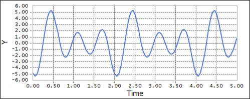
Figure 4.59 Scope result using the FORSIN function
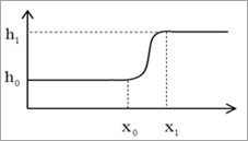
4.7.1.9.5. HAVSIN
The HAVSIN function interpolates between two markers using a trigonometric function. Generally, this function is used to link two markers in a gradual curve, similar to the Step and Step 5 functions.
Format
Arguments definition
\({x}\) |
The input variable for the defined HAVSIN - Generally, this variable is time or a function that returns a real number. |
\({x}_{0}\) |
The starting point for the HAVSIN function |
\({h}_{0}\) |
The initial value for the input variable (within the range of x≤x0) |
\({h}_{1}\) |
The ending point for the HAVSIN function |
\({x}_{1}\) |
The initial value for the input variable (within the range of x≥x1) |
Formulation
\(\begin{aligned} & \text{HAVSIN}={{h}_{0}},\ \,\,\,\,\,\,\,\,\,\,\,\,\,\,\,\,\,\,\,\,\,\,\,\,\,\,\,\,\,\,\,\,\,\,\,\,\,\,\,\,\,\,\,\,\,\,\,\,\,\,\,\,\,\,\,\,\,\,\,\,\,\,\,\,\,\,\,\,\,\,\,\,\,\,\,\,\,\,\,\,\,\,\,\,\text{when }x\le \,{{x}_{0}} \\ & \,\,\,\,\,\,\,\,\,\,\,\,\,\,\,\,\,\,\,\,\,\,=\frac{({{h}_{0}}+{{h}_{1}})}{2}+\frac{({{h}_{1}}-{{h}_{0}})}{2}\,\cdot \sin \left( \pi \frac{(x-{{x}_{0}})}{({{x}_{1}}-{{x}_{0}})}-\frac{\pi }{2} \right)\,,\,\,\,\text{when}\,\,{{x}_{0}}\le x\le {{x}_{1}} \\ & \,\,\,\,\,\,\,\,\,\,\,\,\,\,\,\,\,\,\,\,\,\,={{h}_{1}},\,\,\,\,\,\,\,\,\,\,\,\,\,\,\,\,\,\,\,\,\,\,\,\,\,\,\,\,\,\,\,\,\,\,\,\,\,\,\,\,\,\,\,\,\,\,\,\,\,\,\,\,\,\,\,\,\,\,\,\,\,\,\,\,\,\,\,\,\,\,\,\,\,\,\,\,\,\,\,\,\,\,\,\,\,\,\text{when}\,x\ge {{x}_{1}} \\ \end{aligned}\)
Example
HAVSIN (time, 1.0, 0.0, 4.0, 1.0)
\({x}\) = time: Independent variable
\({x}_{0}\) = 1.0: The x-value at which the HAVSIN function begins
\({h}_{0}\) = 0.0: Initial value of the HAVSIN function
\({x}_{1}\) = 4.0: The x-value at which the HAVSIN function ends
\({h}_{1}\) =1.0 : Final value of the HAVSIN function
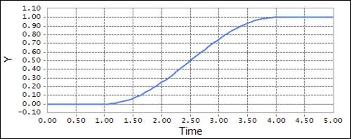
Figure 4.60 Scope result using the HAVSIN function
4.7.1.9.6. IMPACT
The IMPACT function returns the contact force in a contact model defined by the relative location and velocity of two markers.
Format
Arguments definition
Distance(\(x\)) |
The expression for the relative distance between the two markers on the contacting entities |
Velocity(\(\dot{x}\)) |
The expression for the relative velocity between the two markers on the contacting entities |
Freelength(\({{x}_{1}}\)) |
The contact distance between the two markers on the contacting entities - This must be a real number or a function that returns a real number. - The free length(x1) determines whether or not contact is made. |
Stiffness(\(k\)) |
The modulus rigidity on the spring force |
Stiffnessexponent(\(\exp\)) |
The nonlinear coefficient value on the surface of the spring force |
Damping(\({{c}_{\max }}\)) |
The maximum damping coefficient for the calculation of the damping force |
Penetration(\(d\)) |
The depth at which the damping coefficient reaches 0 |
Formulation
\(\begin{aligned} & \text{IMPACT =} \\ & \left\{ \begin{aligned} & k{{({{x}_{1}}-x)}^{\exp }}-\text{STEP}(x,{{x}_{1}}-d,{{c}_{\max }},{{x}_{1}},0)\cdot \dot{x}\,\,\,\,\text{when},\text{ }x<\,{{x}_{1}} \\ & \text{0}\,\,\,\,\,\,\,\,\,\,\,\,\,\,\,\,\,\,\,\,\,\,\,\,\,\,\,\,\,\,\,\,\,\,\,\,\,\,\,\,\,\,\,\,\,\,\,\,\,\,\,\,\,\,\,\,\,\,\,\,\,\,\,\,\,\,\,\,\,\,\,\,\,\,\,\,\,\,\,\,\,\,\,\,\,\,\,\,\,\,\text{when},\text{ }x<\,{{x}_{1}}\And \,\,\text{IMPACT }<0 \\ & 0\,\,\,\,\,\,\,\,\,\,\,\,\,\,\,\,\,\,\,\,\,\,\,\,\,\,\,\,\,\,\,\,\,\,\,\,\,\,\,\,\,\,\,\,\,\,\,\,\,\,\,\,\,\,\,\,\,\,\,\,\,\,\,\,\,\,\,\,\,\,\,\,\,\,\,\,\,\,\,\,\,\,\,\,\,\,\,\,\,\text{when},\text{ }x\ge {{x}_{1}}\,\, \\ \end{aligned} \right. \\ \end{aligned}\)
Example
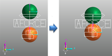
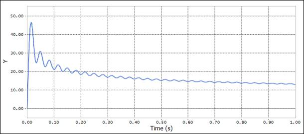
Figure 4.61 Example modeling for the IMPACT function
IMPACT(DY(Body2.Marker1,Body1.Marker2,Body1.Marker2),VY(Body2.Marker1,Body1.Marker2,Body1.Marker2),100,1000,1.3,10,2)
\({x}\) = DY: Distance variable
\({\dot{x}}\) = VY: The time derivative of y
\({x}_{0}\) = 0.0: Free length of y
\({k}\) =1000: Stiffness
\({x}\) = 1.3: Exponent of the force
\({exp}\) = 10: Maximum damping coefficient
\({d}\) = 2: Boundary penetration

Figure 4.62 Scope result using the IMPACT function
4.7.1.9.7. POLY
The POLY function returns the results of the input variables and coefficients evaluated in a polynomial function.
Format
Arguments definition
\({x}\) |
The input variable for the defined polynomial function - Generally, this variable is time or a function that returns a real number. |
\({x}_{0}\) |
The starting point of the polynomial function |
\({a}_{0}, {a}_{1}, \cdots, {a}_{30}\) |
The set of polynomial coefficients (up to 31) |
Formulation
\(\begin{aligned} & \text{POLY}=\sum\limits_{j=0}^{n}{{{a}_{j}}{{(x-{{x}_{0}})}^{j}}}\,\,\,\,\,\,\,\,\,\,\,\,\,\,\,\,\,\,\,\,\,\,\,\,\,\,\,\,\,\,\,\,\,\,\,\,\,\,\,\,\,\,\,\,\text{where, }0\le j\le n \\ & \,\,\,\,\,\,\,\,\,\,={{a}_{0}}+{{a}_{1}}(x-{{x}_{0}})+{{a}_{2}}{{(x-{{x}_{0}})}^{2}}+\cdots +{{a}_{n}}{{(x-{{x}_{0}})}^{n}} \\ \end{aligned}\)
Example
POLY (time, 0, 1,1,1)
\({x}\) = time: Independent variable
\({x}_{0}\) = 0: Shift in the polynomial
\({a}_{0}\), \({a}_{1}\), \({a}_{2}\): Define coefficient for the polynomial series
\({a}_{0}\) = 1, \({a}_{1}\) = 1, \({a}_{2}\) = 1
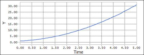
Figure 4.63 Scope result using the POLY function
4.7.1.9.8. SHF
The SHF function returns the results of the input variables and coefficients evaluated as a sine wave in a simple harmonic function.
Format
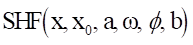
Arguments definition
\({x}\) |
The input variable for the defined SHF function - Generally, this variable is time or a function that returns a real number. |
\({x}_{0}\) |
The starting point of the simple harmonic function |
\({a}\) |
The amplitude value for the sine wave of the variable This value must be a real number or a function that returns a real number |
\({\omega}\) |
The frequency of the simple harmonic function |
\({\phi}\) |
The phase shift value of the simple harmonic function |
\({b}\) |
The average frequency of the simple harmonic function |
Formulation
\(\text{SHF}=a\cdot \sin (\omega \cdot (x-{{x}_{0}})-\phi )+b\)
Example
SHF(time, 10D, PI,360D,0,3)
\({x}\) = time: Independent variable in the function
\({x}_{0}\) = 10D: Offset in the independent variable x
\({a}\) = PI: Amplitude of the harmonic function
\({\omega}\) = 360D: The frequency of the harmonic function
\({\phi}\) = 0: Phase shift in the harmonic function
\({b}\) = 3: Average displacement of the harmonic function
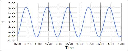
Figure 4.64 Scope result using the SHF function
4.7.1.9.9. STEP
The STEP function interpolates between two markers using a cubic polynomial. Generally, this function is used when linking two markers in a gradual curve.
Format
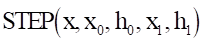
Arguments definition
\({x}\) |
The variable for the defined STEP function - Generally, this variable is time or a function that returns a real number. |
\({x}_{0}\) |
The starting point of the STEP function. |
\({h}_{0}\) |
The initial value for the input variable (within the range of x≤x0) |
\({h}_{1}\) |
The ending point of the STEP function |
\({x}_{1}\) |
The initial value for the input variable (within the range of x≥x1) |
Formulation
\(\begin{aligned} & \text{STEP}={{h}_{0}}\,\,\,,\,\ \,\,\,\,\,\,\,\,\,\,\,\,\,\,\,\,\,\,\,\,\,\,\,\,\,\,\,\,\,\,\,\,\,\,\,\,\,\,\,\,\,\,\,\,\,\,\,\,\,\,\,\,\,\,\,\,\,\,\,\,\,\,\,\,\,\,\,\,\,\,\,\,\,\,\,\,\,\text{when }x\le \,{{x}_{0}} \\ & \,\,\,\,\,\,\,\,\,\,\,\,\,\,=\,\,{{h}_{0}}+({{h}_{1}}-{{h}_{0}}){{\left[ \frac{x-{{x}_{0}}}{{{x}_{1}}-{{x}_{0}}} \right]}^{2}}\left\{ 3-2\frac{x-{{x}_{0}}}{{{x}_{1}}-{{x}_{0}}} \right\}\,,\,\,\,\,\,\text{when }\ {{x}_{0}}\le x\le {{x}_{1}} \\ & \,\,\,\,\,\,\,\,\,\,\,\,\,\,={{h}_{1}}\,\,,\,\,\,\,\,\,\,\,\,\,\,\,\,\,\,\,\,\,\,\,\,\,\,\,\,\,\,\,\,\,\,\,\,\,\,\,\,\,\,\,\,\,\,\,\,\,\,\,\,\,\,\,\,\,\,\,\,\,\,\,\,\,\,\,\,\,\,\,\,\,\,\,\,\,\,\,\,\,\,\,\,\text{when}\,x\ge {{x}_{1}} \\ \end{aligned}\)
Example
STEP(time, 1.0, 0.0, 4.0, 1.0)
\({x}\) = time: Independent variable
\({x}_{0}\) = 1.0: X-value at which the STEP function begins
\({h}_{0}\) = 0.0: Initial value of the STEP function
\({x}_{1}\) = 4.0: X-value at which the STEP functions ends
\({h}_{1}\) = 1.0: Final value of the STEP function
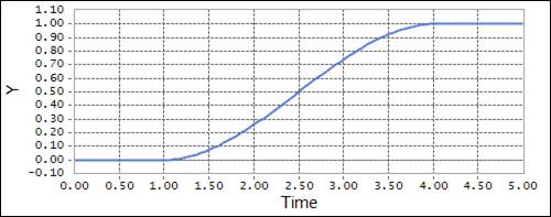
Figure 4.65 Scope result using the STEP function
4.7.1.9.10. STEP5
The STEP5 function interpolates between two markers using a quantic polynomial. Generally, this function is used when linking two markers in a gradual curve.
Format
Arguments definition
\({x}\) |
The input variable for the defined STEP5 function - Generally, this variable is time or a function that returns a real number. |
\({x}_{0}\) |
The starting point of the STEP5 function |
\({h}_{0}\) |
The initial value for the input variable (within the range of x≤x0) |
\({h}_{1}\) |
The ending point of the STEP5 function |
\({x}_{1}\) |
The initial value for the input variable (within the range of x≥x1) |
Formulation
\(\begin{aligned} & \text{STEP5}={{h}_{0}}\,\,\,,\,\ \,\,\,\,\,\,\,\,\,\,\,\,\,\,\,\,\,\,\,\,\,\,\,\,\,\,\,\,\,\,\,\,\,\,\,\,\,\,\,\,\,\,\,\,\,\,\,\,\,\,\,\,\,\,\,\,\,\,\,\,\,\,\,\,\,\,\,\,\,\,\,\,\,\,\,\,\,\,\,\,\,\,\,\,\,\,\,\,\,\,\,\,\,\,\,\,\,\,\,\,\,\,\,\,\,\,\,\,\,\,\,\,\,\text{when }x\le \,{{x}_{0}} \\ & \,\,\,\,\,\,\,\,\,\,\,\,\,\,=\,\,{{h}_{0}}+({{h}_{1}}-{{h}_{0}})\cdot {{\left[ \frac{x-{{x}_{0}}}{{{x}_{1}}-{{x}_{0}}} \right]}^{3}}\cdot \left\{ 10-15\cdot \frac{x-{{x}_{0}}}{{{x}_{1}}-{{x}_{0}}}+6\cdot {{[\frac{x-{{x}_{0}}}{{{x}_{1}}-{{x}_{0}}}]}^{2}} \right\},\,\,\,\text{when }\ {{x}_{0}}<x<{{x}_{1}} \\ & \,\,\,\,\,\,\,\,\,\,\,\,\,\,={{h}_{1}}\,\,,\,\,\,\,\,\,\,\,\,\,\,\,\,\,\,\,\,\,\,\,\,\,\,\,\,\,\,\,\,\,\,\,\,\,\,\,\,\,\,\,\,\,\,\,\,\,\,\,\,\,\,\,\,\,\,\,\,\,\,\,\,\,\,\,\,\,\,\,\,\,\,\,\,\,\,\,\,\,\,\,\,\,\,\,\,\,\,\,\,\,\,\,\,\,\,\,\,\,\,\,\,\,\,\,\,\,\,\,\,\,\,\,\,\,\,\,\,\,\,\text{when}\,x\ge {{x}_{1}} \\ \end{aligned}\)
Example
STEP5(time, 1.0, 0.0, 4.0, 1.0)
\({x}\) = time: Independent variable
\({x}_{0}\) = 1.0: X-value at which the STEP5 function begins
\({h}_{0}\) = 0.0: Initial value of the STEP5 function
\({x}_{1}\) = 4.0: X-value at which the STEP5 functions ends
\({h}_{1}\) = 1.0: Final value of the STEP5 function
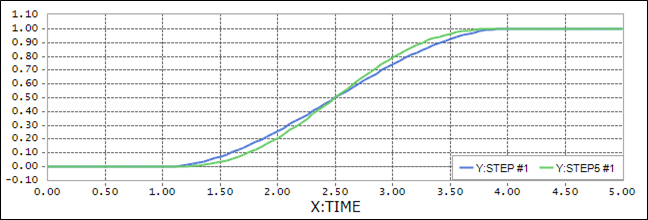
Figure 4.66 Scope result using the STEP vs STEP5 function
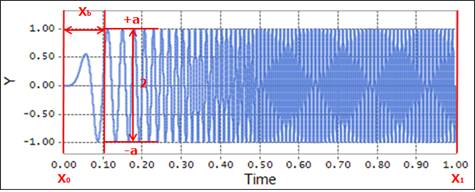
4.7.1.9.11. SWEEP
The SWEEP function returns the results of a regular sine wave function with increasing linear frequency.
Format
Arguments definition
\({x}\) |
Independent variable for the SWEEP function - This variable must be time, a real number, or a function that returns a real number. |
\({a}\) |
Sine function wave |
\({x}_{0}\) |
Starting point of the SWEEP function (x value) |
\({f}_{0}\) |
Initial sine function frequency |
\({x}_{1}\) |
Ending point of the SWEEP function (x value) |
\({f}_{1}\) |
Ending frequency of the sine function |
\({x}_{b}\) |
Range in which the SWEEP function is fully active |
Formulation
\(\begin{aligned} & \text{SWEEP=STEP5}(x,{{x}_{0}},0,{{x}_{0}}+{{x}_{b}},1)\cdot a\cdot \sin (2\pi \cdot \int{freq(x)dx}) \\ & freq(x)=\left\{ \begin{matrix} {{f}_{0}}\,,\,\,\,\,\,\,\,\,\,\,\,\,\,\,\,\,\,\,\,\,\,\,\,\, \\ {{f}_{0}}+\frac{{{f}_{2}}-{{f}_{0}}}{{{x}_{1}}-{{x}_{0}}}\cdot x\,\ ,\ \\ {{f}_{1}},\ \,\,\,\,\,\,\,\,\,\,\,\,\,\,\,\,\,\,\,\,\,\, \\ \end{matrix} \right.\,\ \begin{matrix} \left( \,x\,\,\le \,{{x}_{0}} \right) \\ \left( {{x}_{0}}\ \le \ x<{{x}_{1}} \right) \\ \left( {{x}_{1}}\,\,\le \ x \right) \\ \end{matrix} \\ & \int{freq(x)dx}=\left\{ \begin{matrix} {{f}_{0}}\cdot x\ ,\,\,\,\,\,\,\,\,\,\,\,\,\,\,\,\,\,\,\,\,\,\,\,\,\,\,\,\,\,\,\,\,\,\,\,\,\,\,\,\,\,\,\,\,\,\,\,\,\,\,\,\,\,\,\,\,\,\,\,\,\,\,\,\,\,\,\,\,\,\,\,\,\,\,\,\,\,\,\,\,\,\,\,\,\,\,\,\,\,\,\,\,\, \\ {{f}_{0}}\cdot {{x}_{0}}+{{f}_{0}}\cdot (x-{{x}_{0}})+0.5\frac{{{f}_{1}}-{{f}_{0}}}{{{x}_{1}}-{{x}_{0}}}\cdot {{(x-{{x}_{0}})}^{2}}\ ,\,\,\,\,\,\,\,\,\,\,\,\,\,\,\,\,\,\,\, \\ {{f}_{0}}\cdot {{x}_{0}}+{{f}_{0}}\cdot (x-{{x}_{0}})+0.5\frac{{{f}_{1}}-{{f}_{0}}}{{{x}_{1}}-{{x}_{0}}}\cdot {{({{x}_{1}}-{{x}_{0}})}^{2}}+{{f}_{1}}\cdot (x-{{x}_{0}})\ ,\ \, \\ \end{matrix} \right.\,\begin{matrix} \left( \,x\,\,\le \,{{x}_{0}} \right) \\ \left( {{x}_{0}}\ \le \ x<{{x}_{1}} \right) \\ \left( {{x}_{1}}\,\,\le \ x \right) \\ \end{matrix} \\ \end{aligned}\)
Example
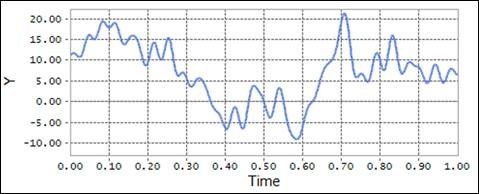
SWEEP(time , 1.0 , 0.0 , 0.0 , 0.5 , 100.0 , 0.1)
\({x}\) = time: Independent variable.
\({a}\) = 1.0: The amplitude of the sinusoidal function.
\({x}_{0}\) = 0.0: X-value at which the SWEEP function begins.
\({f}_{0}\) = 0.0: Initial frequency of the sinusoidal function.
\({x}_{1}\) = 0.5: X-value at which the SWEEP function ends.
\({f}_{1}\) = 100.0: Final frequency of the sinusoidal function.
\({dx}\) = 0.1: Interval value of X-value in which the SWEEP function is fully active.
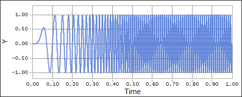
Figure 4.67 Scope result using the SWEEP function
4.7.1.9.12. INVPSD
The INVPSD function returns the results of a time signal from a power spectral density with increasing frequency.
Format

Arguments definition
\({x}\) |
Independent variable for the INVPSD function - This variable must be time, a real number, or a function that returns a real number. |
Spline |
The name or argument number for the spline data defined by the subentity. |
\({f}_{0}\) |
Real value, Minimum frequency for PSD |
\({f}_{1}\) |
Real value, Maximum frequency for PSD |
nFreq |
Integer number that specifies the number of frequencies. This number must be larger than 1 and less than 10000. |
Logarithmic |
Integer number, Logarithmic steps for frequency sampling step of spline data. 0: Linear steps 1: Logarithmic steps for frequency sampling step |
Option |
Integer number, phase option. 0: Random Phase 1: Constant Phase |
Phase |
Real number (=“Phase Option” is 0 or 1 cases). A seed value which generated from the random number for Phase shifts. |
Formulation
\(\begin{aligned} & INVPSD=\sum\limits_{i=1}^{nf}{{{A}_{i}}\cdot \sin (2\pi {{f}_{i}}\cdot x+{{\phi }_{i}})} \\ & \left( \begin{aligned} & where,\,\,\,\,\,Ai=\sqrt{2\cdot (PSD\,data)\cdot df} \\ & \,\,\,\,\,\,\,\,\,\,\,\,\,\,\,\,\,\,\,df=\frac{{{f}_{1}}-{{f}_{0}}}{nFrequency-1} \\ \end{aligned} \right) \\ \end{aligned}\)
This result is summation for a series of sinusoidal functions with the amplitudes which is configured using PSD data from spline curve defined.
The phase value is calculated by a random number generator.
For random phase, there can be difference between rplt data and scope date.
In case of using the same seed value, the each result always is keep the same value.
Example
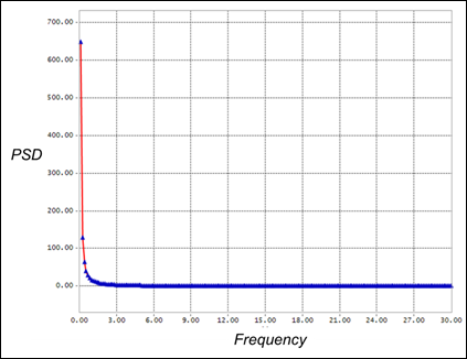
INVPSD (time, sp1, 0.1, 30.0, 199, 0, 0, 0.0)
\({x}\) = time: Independent variable.
Spline = sp1: the spline name.
\({f}_{0}\) = 0.1: Initial frequency of the sinusoidal function.
\({f}_{1}\) = 30.0: Final frequency of the sinusoidal function.
nFreq = 199: the number that specifies the number of frequencies.
Logarithmic = 0: Linear Logarithmic steps for frequency sampling step of spline data.
Option = 0: phase option for random phase shift.
Phase = 0.0: A seed value which generated from the random number for Phase shifts.