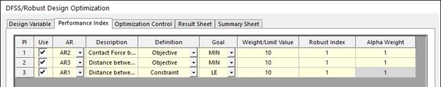
21.3.6.1. Robust Design Optimization

Now, one tries to minimize the performance modified as:

Minimize

(21.1)\[\alpha \cdot f\left( \mathbf{x} \right)+{{k}_{0}}\cdot {{\sigma }_{0}}\left( \mathbf{x} \right)\]

where \(f\left( \mathbf{x} \right)\) and \({{\sigma }_{0}}\left( \mathbf{x} \right)\) are the performance and its variation according to the design variable variation \(\mathbf{\delta }\). Also, the coefficients \(\alpha\) and \({{k}_{0}}\) denotes the weighting factors for them. In AutoDesign, \(\alpha\) and \({{k}_{0}}\) are called as the alpha weight and the robust index for objective, respectively. If one tries to minimize only the variance, he just set \(\alpha =0\) and \({{k}_{0}}=1\).

AutoDesign uses the following \({{\sigma }_{0}}\left( \mathbf{x} \right)\) during optimization process:

(21.2)\[{{\tilde{\sigma }}_{0}}\left( \mathbf{x} \right)\approx \sqrt{\sum\limits_{i=1}^{n}{\left( {{\left| \frac{\partial f\left( \mathbf{x} \right)}{\partial {{x}_{i}}} \right|}^{2}}\delta _{i}^{2} \right)+...}}\]

which is similar to Taylor series approximation for a variance in statistics. If \({{\delta }_{i}}={{\sigma }_{i}}\) for each design variable, then \({{\tilde{\sigma }}_{0}}\left( \mathbf{x} \right)\) is the approximate standard deviation of \(f\left( \mathbf{x} \right)\) directly. As one may not know \({{\sigma }_{i}}\) in the practical design, he or she uses the variation \({{\delta }_{i}}\) simply. This represents that \({{\tilde{\sigma }}_{0}}\left( \mathbf{x} \right)\) can be a variation for \(f\left( \mathbf{x} \right)\), even though it is not the approximation of standard deviation.

What is a robust design for constrained optimization problem? Now, consider the robust design for it. First, let’s consider the equality constraints. Suppose that an equality constraint \({{h}_{i}}\left( \mathbf{x} \right)=0\) is transformed into \({{h}_{i}}\left( \mathbf{x} \right)\pm {{\sigma }_{i}}\left( \mathbf{x} \right)=0\) as a robust design formulation. From the definition of equality constraint, this transformed constraint is satisfied only when \({{\sigma }_{i}}\left( \mathbf{x} \right)=0\). It is unusual in the practical design problem. Thus, one equality constraint can be divided into two inequality constraints as:

(21.3)\[\begin{split}\left| {{h}_{i}}\left( \mathbf{x} \right) \pm {{\sigma }_{i}}\left( \mathbf{x} \right) \right|\le {{\varepsilon }_{i}}\to \left\{ \begin{matrix} {{h}_{i}}\left( \mathbf{x} \right)+{{\sigma }_{i}}\left( \mathbf{x} \right)\leq {{\varepsilon }_{i}} \\ {{h}_{i}}\left( \mathbf{x} \right)-{{\sigma }_{i}}\left( \mathbf{x} \right) \geq -{{\varepsilon }_{i}} \end{matrix} \right\}\end{split}\]

where, \({{\varepsilon }_{i}}\) is a limit value defined by user. If a robust design formulation is required for equality constraint, AutoDesign recommends that the user divide it into two inequality constraints. Thus, when you define an equality constraint in the window of Robust Design Optimization in AutoDesign, Robust Index column are deactivated automatically.

Second, let’s consider a robustness of inequality constraints. AutoDesign has two types of inequality constraints such as ‘less than \(\left( {{g}_{j}}\left( \mathbf{x} \right)\le {{\varepsilon }_{j}} \right)\)’ and ‘greater than \(\left( {{g}_{j}}\left( \mathbf{x} \right)\ge {{\varepsilon }_{j}} \right)\)’ types. Their robust formulations are represented as:

(21.4)\[{{g}_{j}}\left( \mathbf{x} \right)+{{\sigma }_{j}}\left( \mathbf{x} \right)\le {{\varepsilon }_{j}} \text{and} {{g}_{j}}\left( \mathbf{x} \right)-{{\sigma }_{j}}\left( \mathbf{x} \right)\ge {{\varepsilon }_{j}}\]

where, \({{\sigma }_{j}}\left( \mathbf{x} \right)\) can be evaluated similarly as (21.2). Figure 21.81 shows the feasibility between a nominal optimum and a robust optimum.

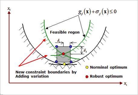
Figure 21.81 Robust design for inequality constraints

When the final design (\({{\mathbf{x}}^{*}}\)) has variations within \({{\mathbf{x}}^{*}}\pm \mathbf{\delta }\), the final design is a robust optimum if all the sampled responses \({{g}_{j}}\left( {{\mathbf{x}}^{*}}\pm \mathbf{\delta } \right)\) are in the feasible region while optimizing its’ objective.