3.5.7.1. General Page
These options provided on this page are for RecurDyn/Solver.
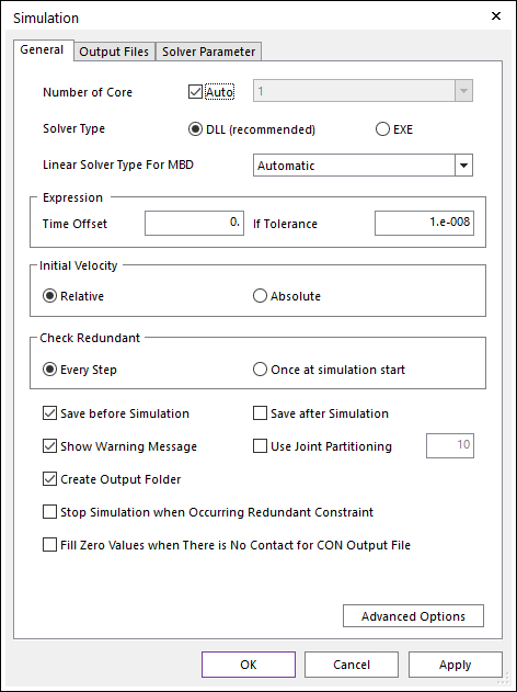
Figure 3.92 Simulation dialog box [General]
Number of Core: Specifies the number of parallel threads. RecurDyn/Solver uses the specified threads as much as possible for fast solving.
Auto
If this option is checked, the number of threads is automatically selected.
If this option is not checked, the user can choose one in the drop-down menu containing 1,2,4,8, and 16 CPU cores. RecurDyn/Solver supports cores up to 16. However, to use more than 4, SMP licenses are needed.
The entities supported in this option are as follows.
Product
Entities
Professional
Sphere To Sphere Contact
Sphere To Cylinder Contact
Cylinder In Cylinder Contact
Cylinder To Cylinder Contact
Cone To Cylinder Contact
Sphere To Cone Contact
Cone In Cone Contact
Cone To Cone Contact
Circle To Circle Contact
Sphere In Sphere Contact
Sphere To Box Contact
Sphere To Torus Contact
Sphere In Torus Contact
Sphere In Cylinder Contact
Sphere To Arc Revolution Contact
Sphere To Arc Extrusion Contact
Geo Surface Contact
Geo Sphere Contact
Geo Cylinder Contact
Geo Curve To Surface Contact
UV Sphere Contact
Geo Curve 3D Contact
Geo Sphere To Curve 3D Contact
Geo Curve Contact
Geo Circle Contact
Bushing Force
Beam Force
Plate Force
FFlex
All elements
MTT2D
Flexible Rollers
MTT3D
Shell Sheet
R2R2D
Beam Assembly
Belt
Beam Belt
Shell Belt
Chain
Assembly
Gear
Involute Analytic Contact
Track LM
Assembly
Track HM
Assembly
Note
Using many cores does not mean that the analysis time can be reduced. You simulate the model that is not suitable for multi-thread as multi-thread and uses the entire CPU, while Turbo Boost is turned off and the CPU clock drops, which slows the analysis time.
When using KISSsoft Direct Contact of Drivetrain Gear, CPU is used at 100% regardless of Core selection. This is because KISSsoft is an external program and RecurDyn cannot control its CPU Setting.
Solver Type
DLL(recommend): Selects the solver type to launch a DLL version of the solver. It runs in the fastest simulation time. (This option is the default.)
EXE: Selects the solver type which is the separate process using an EXE file. The EXE option is used with large models where the solver memory should be considered. When selecting the EXE solver type, RecurDyn/Solver does not share any memory with RecurDyn/Modeler.
Linear Solver Type For MBD
Automatic: This option changes the option to DENSE or SPARSE depending on the size of the system matrix for MBD. If the size of the system matrix for MBD is less than or equal to 1000, it is set to DENSE, and if larger, to SPARSE. (The size of the system matrix for MBD is determined by the sum of generalized coordinates, the number of constraints, the number of variable equations, the number of differential equations, and the number of RFlex mode shapes) (This option is the default.)
Dense: Selects the linear solver type to DENSE for MBD system. This option is suitable for below 1000 system matrix sizes.
Sparse: Selects the linear solver type to SPARSE for MBD system. This option is suitable for over 1000 system matrix sizes.
Expression
Time Offset: Makes the TIME function delay as much as the defined value. Generally, the default value is 0. However, in the case of the extracted model, this value should be changed to the time to execute the Extract function in a model which has Time variables in the Expressions.
If Tolerance: This is a parameter that modifies the conditions so that the IF function can check the zero condition reasonably. It affects the specific range to be decided as zero.
Initial Velocity
Relative: Initial velocities of a body are imposed as a higher priority when both a body and a joint have the initial velocity at the same time. (This option is the default.)
Absolute: Initial velocities of a joint are imposed even though the initial velocity of a body has been already defined. In other words, the initial velocity of the body is neglected when simulating a model.
Check Redundant
Every Step: Checks redundant constraints for every step. (This option is the default.)
Once at Simulation Start: Checks redundant constraints just only once at the early stage of the analysis.
Save before Simulation: If this option is checked, the model is saved just before executing the simulation. (The default option is checked.)
Save after Simulation: If this option is checked, the model is saved just after executing the simulation. (The default option is unchecked.)
Show Warning Massage: If this option is checked, the warning messages appear in the Message Window (The default option is checked.). If this option is not checked, the warning messages are not displayed in the Message Window.
Use Joint Partitioning: If this option is checked, to improve the solving speed, it makes the calculating matrix size reduced by the user-defined input, which should be greater than or equal to 10, and less than or equal to 50. This option is effective when the MBD model has dozens of Joints such as the MTT2D sheet.
Create Output Folder: If this option is checked, an output folder is created before the simulation. This option also applies to CoLink. Whenever performing the simulation, the output folder is generated sequentially (The default is checked.). If this option is not checked, an output folder is not created and the result files are generated in the same location where *.rdyn exists.
Stop Simulation when Occurring Redundant Constraint: If this option is checked, the simulation is stopped when redundant constraints occur.
Fill Zero Values when There is No Contact for CON Output File: If this option is checked, when there is no contact point on the step, zero values are written in the Contact Information File (*.con) that is created from Solid Contact, Geo Contact, and UV Sphere Contact.
Advanced Options
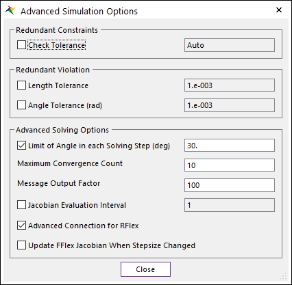
Figure 3.93 Advanced Simulation Options dialog box
Redundant Constraints
A numerical tolerance is used inside of the RecurDyn/Solver to determine which constraints are redundant. If Check Tolerance is not checked, then RecurDyn automatically uses the value of 1e-4 for the numerical tolerance. In some cases, the automatic tolerance value can be too large. When that happens, RecurDyn treats too many constraints as redundant constraints. Redundant constraints are removed from the simulation.
Check Tolerance: If this option is checked, the user can specify a tolerance value manually. The tolerance value must be greater than zero. When the user selects to Include in Position and Velocity Pre-Analysis, sometimes, the automatic tolerance is too large. In this case, it is recommended that the user set a smaller tolerance. In the case of FFlex bodies that are included in the pre-analysis, when the tolerance is too large, RecurDyn does not adjust the positions of the FFlex bodies to match the initial conditions set by the user.
Redundant Violation
Redundant constraints are removed from the simulation. But the value of redundant constraints has to be checked because some constraint violation occurs in the case of incompatible redundant constraints.
Length Tolerance: If this option is checked, the user can specify a tolerance value for the length manually. If redundant constraints are over the tolerance, the simulation is stopped. If a tolerance value is a negative number, the simulation is stopped if there are any redundant constraints.
Angle Tolerance: If this option is checked, the user can specify a tolerance value for the angle manually. If redundant constraints are over the tolerance, the simulation is stopped. If a tolerance value is a negative number, the simulation is stopped if there are any redundant constraints.
Advanced Solving Options
Limit of Angle in each Solving Step: If this option is checked, the angle which can be moved in one step is limited. It is helpful for more accurate analysis for high-speed rotational problems. Too fast rotation can cause inaccurate result. This option limits the angle of the rotation during one step so that it reduces the step size to improve accuracy. So, even if the user uses the big maximum step size, the solver adjusts the step size according to the amount of the rotation, so that it gives a positive effect on the simulation speed.
Maximum Convergence Count: Defines the number of counts used to increase the step size. The number of counts means how many convergence counts are needed to increase the step size. If this value is 1, then just 1 successful convergence increases the step size, so that the simulation speed can become faster. But it can cause instability in the simulation as a side effect.
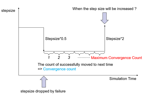
Figure 3.94 Maximum Convergence Count
Message Output Factor: Solving message (simulation n time, Step size, NJAC, NRES, ANRF, and, AINTF) writing period can be changed this option. There is a count for this function in the integrator. The count is counted whenever successfully moving the next time step. If the count is reaching to the Message Output Factor, then solving message is written and the count is triggered to zero. The default is 100. Range: (1~100000)
Jacobian Evaluation Interval: If this option is checked, the user can modify Jacobian Evaluation Interval manually. This option controls the frequency to calculate the Jacobian during simulation. If the change in the behavior of the model is not big, the simulation speed can be improved by using the bigger interval (> 1).
NJAC written in the message window means the accumulated number of the Jacobian evaluation.
In the below case, 100->199 means the Jacobian was calculated 99 times. If this variation is similar to the Message Output Factor (the default is 100), we can assume that Jacobian doesn’t change a lot. In this case, the simulation speed can be improved by using the bigger Jacobian Evaluation Interval. (But it can lower the accuracy, so you need to be careful when you change this value)
The default value is 1.
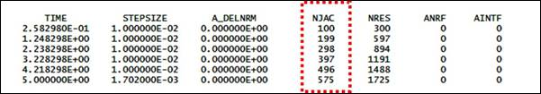
Figure 3.95 Message Window
Advanced Maximum Stepsize Factor: This option affects the model if there are multiple contacts in the model and the MSSF (Maximum Stepsize Factor) values applied to each contact are different. If this option is checked, at the time of analysis, the solver reduces the step size using the largest MSSF value among the contacts that the contact boundary is likely to meet. If this option is off, the solver reduces the step size using the largest MSSF value among all contacts.
Advanced Connection for RFlex: This option affects an RFlex system with connectors (force or joint). If this option is checked on, the virtual joint created between the RFlex body and connector is changed to constraint.
Update FFlex Jacobian When Stepsize Changed: This option affects every FFlex system. If this option is checked on, FFlex Jacobian is updated whenever step size is changed.