5.16.3. State Matrix

RecurDyn model includes the plant model, the plant inputs and the plant outputs as Figure 5.132.

Figure 5.132 Multi Body System

RecurDyn/Linear carries out linearization of plant model.

The linearized equation of plant model become

(5.42)\[\hat{\mathbf{M}}\delta\ddot{\mathbf{q}_I}+\hat{\mathbf{C}}\delta\dot{\mathbf{q}_I}+\hat{\mathbf{K}}\delta\mathbf{q}_I=\underline{\mathbf{U}}\]

We define states as

(5.43)\[\begin{split}\underline{\mathbf{X}}=\left[ \begin{matrix} \delta\dot{\mathbf{q}_I} \\ \delta{\mathbf{q}_I} \end{matrix}\right], \underline{\dot{\mathbf{X}}}=\left[ \begin{matrix} \delta\ddot{\mathbf{q}_I} \\ \delta\dot{\mathbf{q}_I} \end{matrix}\right]\end{split}\]

From (5.42), the A matrix and B matrix can be derived as below equation

\[\begin{split}\underline{\dot{\mathbf{X}}}=\left[ \begin{matrix} \hat{\mathbf{M}}^{-1}\hat{\mathbf{C}} & \hat{\mathbf{M}}^{-1}\hat{\mathbf{K}} \\ \mathbf{I} & \mathbf{0} \end{matrix} \right] \underline{\mathbf{X}} + \left[ \begin{matrix} \hat{\mathbf{M}}^{-1}\mathbf{I} \\ \mathbf{0} \end{matrix} \right]\underline{\mathbf{U}}\end{split}\]

\[\begin{split}\underline{\mathbf{A}}=\left[ \begin{matrix} -\hat{\mathbf{M}}^{-1}\hat{\mathbf{C}} & -\hat{\mathbf{M}}^{-1}\hat{\mathbf{K}} \\ \mathbf{I} & \mathbf{0} \end{matrix}\right]\end{split}\]

(5.44)\[\begin{split}\underline{\mathbf{B}}=\left[ \begin{matrix} \hat{\mathbf{M}}^{-1}\hat{\mathbf{I}} \\ \mathbf{0} \end{matrix}\right]\end{split}\]

Plant outputs are defined the function of \(\mathbf{q}_I\), \(\dot{\mathbf{q}}_I\), \(\mathbf{U}\)

(5.45)\[\underline{\mathbf{Y}}=\underline{\mathbf{C}}\underline{\mathbf{X}}+\underline{\mathbf{D}}\underline{\mathbf{U}}\]

Conclusively, in State Matrix the linearized RecurDyn model is represented as:

(5.46)\[\begin{split}\underline{\dot{\mathbf{X}}}=\underline{\mathbf{A}}\underline{\mathbf{X}}+\underline{\mathbf{B}}\underline{\mathbf{U}} \\ \underline{\mathbf{Y}}=\underline{\mathbf{C}}\underline{\mathbf{X}}+\underline{\mathbf{D}}\underline{\mathbf{U}}\end{split}\]

Where:

\(\dot{\mathbf{X}}\) represents the state variables of the plant.

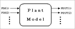
\(\mathbf{U}\) represents the plant inputs.

\(\mathbf{Y}\) represents the plant outputs.

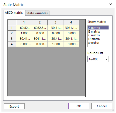
\(\mathbf{A}\), \(\mathbf{B}\), \(\mathbf{C}\) and \(\mathbf{D}\) are state matrices.

You can define the plant inputs and plant outputs. RecurDyn/Solver automatically determines the states. But if you want to make arbitrary coordinate states, you change states by modeling plant input force in the arbitrary coordinate.

Step to Operate State Matrix

1. Check the Included State Matrix option in the Pre-Analysis dialog box, the Static Analysis dialog box, the Dynamic/Kinematic Analysis dialog box.

2. Simulate the model.

3. Click State Matrix icon of the Post Tool group in the Analysis tab.

4. View state matrices.

   

   Figure 5.133 State Matrix dialog box

   • x vector: Initial conditions for the state variables.