21.3.9.2. Interpretation of Monte-Carlo Simulation Results

We provide two result sheets such as Result Sheet and Summary Sheet. Figure 21.117 shows Result Sheet. In this sheet, you can see the sampling points and the probability distribution of performance index. When you see the sample points, first select two design parameters and push Draw button. Then, you can see scattered points. Similarly, you can see the probability of the limit state function values (Performance Index values). In the probability distribution, minus (-) valued performance index (horizontal axis) denote failure zone.

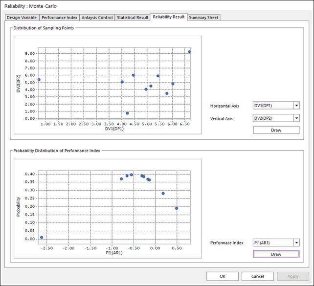
Figure 21.117 Result Sheet of Monte-Carlo simulation

Although two constraint types are provided such as Greater Than and Less Than, the internal solver use Greater Than type constraint as a standard form. Thus, Less Than type constraints are internally transformed into Greater Than type constraints. Also, they are normalized by using their limit values.

Internal Conversion of Performance Index:

\(\bar{P}I=\frac{AR}{LimitValue}-1\) for GE type

\(\bar{P}I=1-\frac{AR}{LimitValue}\) for LE type

As the constraint is .LE. type in this problem, the internal performance index is transformed as

\(\bar{P}I=1-\frac{AR(1)}{36}\)

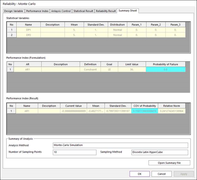
Figure 21.118 Summary Sheet of Monte-Carlo simulation

Figure 21.118 shows the summary sheet. In this sheet, the statistical information for random variables is listed. The values of Param_1 ~ Param_3 are parameters that represent the probabilistic distribution, which are internally calculated. Table 21.5 lists those parameters. The detailed information of those parameters is explained in Probability Distributions.

Table 21.5 Statistical Parameters for probabilistic distribution

	Log-Normal	EVD-I	EVD-II	EVD-III (Max)	EVD-III (Min)	Weibull	Uniform	Beta
Param_1	\(\sigma_Y\)	\(a\)	\(\nu\)	\(a\)	\(a\)	\(\nu\)	\(a\)	\(q\)
Param_2	\(\mu_Y\)	\(w\)	\(k\)	\(m\)	\(m\)	\(m\)	\(b\)	\(r\)
Param_3	-	-	-	\(w\)	\(\varepsilon\)

The goal of Monte-Carlo simulation, failure property is listed in Performance Index (Formulation). In this problem, the failure of probability is obtained as 0.8 (80%).

In Performance Index (Result), Current Value is PI value for the given mean values. Mean and Standard Dev are sample mean and sample standard deviation for PI values evaluated at sampled points. ‘COV of Probability’ is an important measure of Monte-Carlo simulation validation, which are evaluated as

\(COV({{P}_{f}})\approx \frac{\sqrt{\frac{(1-{{P}_{f}}){{P}_{f}}}{N}}}{{{P}_{f}}}\)

The value of \({{P}_{f}}\) is failure probability, \(N\) is number of sampled points. Smaller value of COV represents that the Monte-Carlo simulation gives more accurate result. ‘Relative Norm’ represents the normalized difference between ‘Current Value’ and Mean. Next, we compares the accuracy of Monte-Carlo simulation by increasing the number of sample points.

Let’s consider the following Adaptive Monte-Carlo Simulation concept. For more accurate estimation, we uses 20 sample points (new 10 points + 10 points get from simulation history). To do this, check New Sampling and enter 10 in the column Number of Sampling points. Next, check Get From Simulation History and get the 10 analysis results

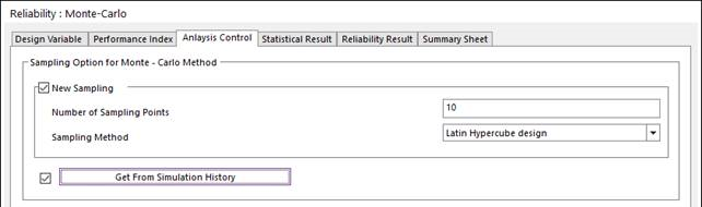
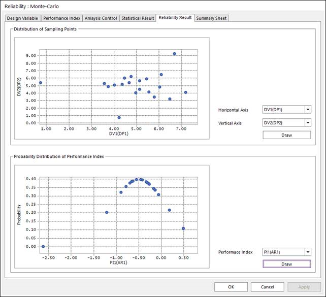
Figure 21.119 Result Sheet for 20 sample points from 20 sample points

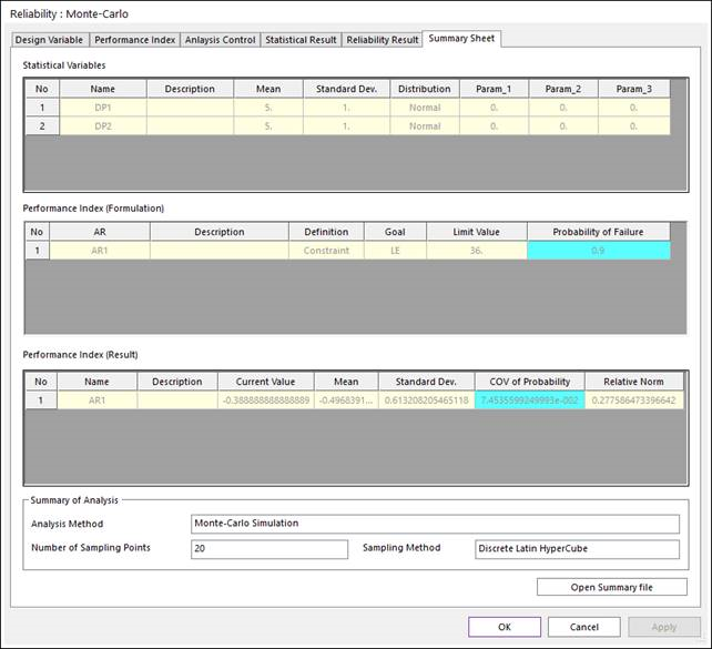
Figure 21.120 Summary Sheet for 20 sample points from 20 sample points

Figure 21.119 and Figure 21.120 show the analysis results for 20 sample points, respectively. Two figures show that failure probabilities converge from 0.8 to 0.9. Also, the COV values are sequentially reduced from 10 sample points (shown in Figure 21.119) to 20 sample points (shown in Figure 21.120).