11.2.1. Background

In order to create a RFlex body in RecurDyn, a RFI file must be needed. The RFI file is the reduced-flexible body interface file which contains a FE-mesh data such as nodes, elements, properties and materials. In addition, it has the eigenvalue results (frequencies) and the eigenvector results (mode shapes, stress shapes, strain shapes) and invariant variables.

There are two types to perform the reduction analysis as CMS and the Normal Mode analysis. At that time, the type of mass matrix must be a lumped mass. The relationship of a mode shape and a global mass matrix is as follows.

\({{\boldsymbol{\Phi }}^{T}}\mathbf{M\Phi }=\mathbf{I}\)

And also, the relationship of a mode shape and a global stiffness matrix is as follows.

\({{\mathbf{\Phi }}^{T}}\mathbf{K\Phi }=Diagonal(\omega _{1}^{2},\omega _{2}^{2},\cdots \omega _{nM}^{2})\)

Where, \(\omega _{j}^{2}\) is an eigenvalue for \(j\) -th mode.

The eigenvalue \(\omega _{j}^{2}\) can be converted a frequency using following equation.

\({{f}_{j}}=\cfrac{\sqrt{\omega _{j}^{2}}}{2\pi }\).

11.2.1.1. CMS Analysis

Component Mode Synthesis (CMS) is a well-known reduction method. And Craig-Bampton method [Ref.1] is another name of CMS. The Craig-Bampton mode is combination of a constraint mode and a fixed-interface normal mode.

\(\mathbf{\Phi }=\left[ \begin{matrix} \mathbf{I} & \mathbf{0} \\ {{\boldsymbol{\Psi }}_{c}} & {{\boldsymbol{\varphi }}_{n}} \\ \end{matrix} \right]\)

The first column is a constraint mode. And the last column is a fixed interface normal mode. Therefore, the number of CMS modes is (Interface DOFs + No. Fixed interface normal modes).

Constraint mode

The constraint mode is computed as the following condition.

\(\left[ \begin{matrix} {{\mathbf{K}}_{cc}} & {{\mathbf{K}}_{cn}} \\ {{\mathbf{K}}_{nc}} & {{\mathbf{K}}_{nn}} \\ \end{matrix} \right]\left[ \begin{matrix} \mathbf{1} \\ {{\mathbf{\Psi }}_{c}} \\ \end{matrix} \right]=\left[ \begin{matrix} \mathbf{R} \\ \mathbf{0} \\ \end{matrix} \right]\)

Where, \(c\) means DOFs for interface nodes, n means the other DOFs except for interface nodes.

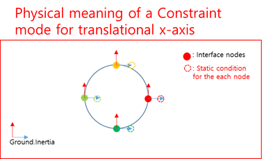
Figure 11.29 Physical meaning of a constraint mode

Constraint mode with a special coordinate system

The constraint mode is computed as the following condition.

\(\left[ \begin{matrix} {{\mathbf{K}}_{cc}} & {{\mathbf{K}}_{cn}} \\ {{\mathbf{K}}_{nc}} & {{\mathbf{K}}_{nn}} \\ \end{matrix} \right]\left[ \begin{matrix} \mathbf{A} \\ \mathbf{\Psi }_{c}^{*} \\ \end{matrix} \right]=\left[ \begin{matrix} \mathbf{R} \\ \mathbf{0} \\ \end{matrix} \right]\)

Where, \(c\) means DOFs for interface nodes, n means the other DOFs except for interface nodes. \(A\) means an orientation matrix (a matrix 3 \(\times\) 3, and consist of direction cosine vectors).

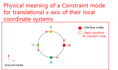
Figure 11.30 Physical meaning of a constraint mode with a special coordinate system

Fixed interface normal mode

The fixed interface normal mode is computed the following eigenvalue equation.

\(({{\mathbf{K}}_{nn}}-\boldsymbol{\lambda }{{\mathbf{M}}_{nn}})\boldsymbol{\varphi }=\mathbf{0}\)

The computed eigenvectors must be following the condition called as the orthonormalization with the mass matrix.

\(\boldsymbol{\varphi }_{n}^{T}{{\mathbf{M}}_{nn}}{{\boldsymbol{\varphi }}_{n}}=\mathbf{I}\)

Orthonormalization

The Craig-Bampton mode is not directly used. Because, the mode shape of RecurDyn/RFlex must be an orthonormalization with the global mass matrix. A transformation matrix \({{\boldsymbol{\Phi }}^{*}}\) is needed for the orthonormalization like following equation.

\(\begin{aligned}& \mathbf{\Phi }={{\mathbf{\Phi }}_{CB}}{{\mathbf{\Phi }}^{*}}\quad \left( {{\mathbf{\Phi }}_{CB}}=\left[ \begin{matrix} \mathbf{I} & \mathbf{0} \\ {{\boldsymbol{\Psi }}_{c}} & {{\boldsymbol{\varphi }}_{n}} \\ \end{matrix} \right] \right) \\ & {{\mathbf{\Phi }}^{T}}\mathbf{M\Phi }={{\left( {{\mathbf{\Phi }}_{CB}}{{\mathbf{\Phi }}^{*}} \right)}^{T}}\mathbf{M}{{\mathbf{\Phi }}_{CB}}{{\mathbf{\Phi }}^{*}}=\mathbf{I} \\ & {{\mathbf{\Phi }}^{T}}\mathbf{K\Phi }={{\left( {{\mathbf{\Phi }}_{CB}}{{\mathbf{\Phi }}^{*}} \right)}^{T}}\mathbf{K}{{\mathbf{\Phi }}_{CB}}{{\mathbf{\Phi }}^{*}}=Diagonal(\omega _{1}^{2},\omega _{2}^{2},\cdots \omega _{nM}^{2}) \\ \end{aligned}\)

Reference,

[Craig1968]

Craig R. R. and Bampton M. C. C., “Coupling of Substructures for Dynamic Analysis”, AIAA Journal, vol. 6, PP. 1313-1319., 1968

11.2.1.2. Normal Mode Analysis

The normal mode analysis is a simple eigenvalue problems using a global stiffness matrix and a global mass matrix as following equation.

\((\mathbf{K}-\mathbf{\boldsymbol{\lambda} M})\mathbf{\Phi }=\mathbf{0}\)

The mode shape must be as the orthonormalization with the global mass matrix.