21.3.5.1. Mathematical Formulation of Multi-Objective

In general, numerical optimization, multi-objective is transformed into a single functional called as a preference function. There are several types of preference function such as weighed summation type, weighted distance type and weighted min-max type.

• Weighted Summation Type

  \(P\left( \mathbf{x} \right)=\sum\limits_{i=1}^{m}{{{w}_{i}}\left( \frac{{{f}_{i}}\left( \mathbf{x} \right)-f_{i}^{*}}{f_{i}^{*}} \right)},\text{ }\sum\limits_{i=1}^{m}{{{w}_{i}}}=1\)

• Weighted Distance Type

  \(P\left( \mathbf{x} \right)={{\left( \sum\limits_{i=1}^{m}{{{w}_{i}}{{\left( \frac{{{f}_{i}}\left( \mathbf{x} \right)-f_{i}^{*}}{f_{i}^{*}} \right)}^{r}}} \right)}^{\frac{1}{r}}},\text{ }\sum\limits_{i=1}^{m}{{{w}_{i}}}=1\)

• Min-Max Type

  \(P\left( \mathbf{x} \right)=\underset{i=1,2,...,m}{\mathop{\max }}\,\left\{ {{w}_{i}}\left( \frac{{{f}_{i}}\left( \mathbf{x} \right)-f_{i}^{*}}{f_{i}^{*}} \right) \right\},\text{ }\sum\limits_{i=1}^{m}{{{w}_{i}}}=1\)

Conceptually, each local optimum \({{f}_{i}}\left( \mathbf{x}_{i}^{*} \right)\) is preferred as a \(f_{i}^{*}\) in the above formulations. In practical design, no one knows them until solving each single objective optimization. One guesses them properly or replaces them as \({{{f}_{i}}\left( \mathbf{x} \right)}/{{{f}_{i}}\left( \mathbf{x}_{i}^{0} \right)}\;\), where \(\mathbf{x}_{i}^{0}\) is the initial design point.

Now, we compare the optimization results for multi-objective formulations. Suppose that \({{f}_{1}}\left( x \right)={{\left( x-2 \right)}^{2}}\) and \({{f}_{2}}\left( x \right)=5{{\left( x-6 \right)}^{2}}\) is minimized simultaneously. Figure 21.79 shows them.

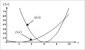
Figure 21.79 Graphical representation of two objectives

If the same weightings are used in these two objectives, Figure 21.79 shows that the pareto optimum is \({{x}^{*}}=4.76393\) and \({{f}_{1}}\left( {{x}^{*}} \right)={{f}_{2}}\left( {{x}^{*}} \right)=3.8196\).

• Weighted Summation Type

  \(\begin{aligned} & P\left( x \right)={{w}_{1}}{{f}_{1}}\left( x \right)+{{w}_{2}}{{f}_{2}}\left( x \right) \\ & =0.5{{\left( x-2 \right)}^{2}}+2.5{{\left( x-6 \right)}^{2}} \end{aligned}\)

  As the optimum satisfies \(\frac{dp}{dx}=0\), it gives

  \(6x-32=0\)

  Thus, the optimum is \({{x}^{*}}=5.3333\), which is different from the Pareto optimum.

• Weighted Distance Type

  Let the value of \(r\) be 2. Then, the distance function is

  \(\begin{aligned} & P\left( x \right)=\sqrt{\left( {{w}_{1}}{{f}_{1}}{{\left( x \right)}^{2}}+{{w}_{2}}{{f}_{2}}{{\left( x \right)}^{2}} \right)} \\ & =\sqrt{0.5{{\left( x-2 \right)}^{4}}+12.5{{\left( x-6 \right)}^{4}}} \end{aligned}\)

  By solving \(\frac{dp}{dx}=0\),

  \(\frac{{{(x-2)}^{3}}+25{{(x-6)}^{3}}}{\sqrt{0.5{{\left( x-2 \right)}^{4}}+12.5{{\left( x-6 \right)}^{4}}}}=0\)

  This gives that \({{x}^{*}}=4.9806\), which is different from the Pareto optimum.

• Weighted Min-Max Type

  \(\begin{aligned} & P\left( x \right)=\max \left\{ {{w}_{1}}{{f}_{1}}\left( x \right),{{w}_{2}}{{f}_{2}}\left( x \right) \right\} \\ & =\max \left\{ 0.5{{\left( x-2 \right)}^{2}},2.5{{\left( x-6 \right)}^{2}} \right\} \end{aligned}\)

  This functional is a composite non-smooth function as follows:

  

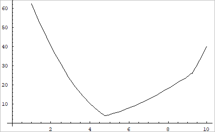
Figure shows that this formulation gives the Pareto optimum \({{x}^{*}}=4.76393\) but it requires some special techniques to overcome the non-smoothness of functional. This is the reason that the min-max type is not used in the gradient-based optimization, even though it can guarantee a local Pareto optimum.