4.11.1. Example for Differential Equation

Description for example model

The user can model differential equations for model such as spring system using DE.

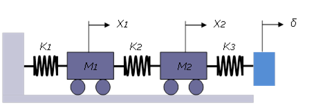
Figure 4.141 Example model

The differential equation for the above example model is as follows:

The model is defined as following equation.

\(\left| \begin{matrix} m1 & 0 \\ 0 & m2 \\ \end{matrix} \right|\left| \begin{matrix} {{{\ddot{x}}}_{1}} \\ {{{\ddot{x}}}_{2}} \\ \end{matrix} \right|+\left| \begin{matrix} {{k}_{1}}+{{k}_{2}} & -{{k}_{2}} \\ -{{k}_{2}} & {{k}_{2}}+{{k}_{3}} \\ \end{matrix} \right|\left| \begin{matrix} {{x}_{1}} \\ {{x}_{2}} \\ \end{matrix} \right|=\left| \begin{matrix} {{F}_{1}} \\ {{F}_{2}}+{{k}_{3}}\delta \\ \end{matrix} \right|\)

And transform 2nd order differential equation to 1st order one.

\(\left[ \begin{matrix} {{m}_{1}} & 0 & 0 & 0 \\ 0 & {{m}_{2}} & 0 & 0 \\ 0 & 0 & 1 & 0 \\ 0 & 0 & 0 & 1 \\ \end{matrix} \right]\left[ \begin{matrix} {{{\ddot{x}}}_{1}} \\ {{{\ddot{x}}}_{2}} \\ {{{\dot{x}}}_{1}} \\ {{{\dot{x}}}_{2}} \\ \end{matrix} \right]+\left[ \begin{matrix} 0 & 0 & {{k}_{1}}+{{k}_{2}} & -{{k}_{2}} \\ 0 & 0 & -{{k}_{2}} & {{k}_{2}}+{{k}_{3}} \\ -1 & 0 & 0 & 0 \\ 0 & -1 & 0 & 0 \\ \end{matrix} \right]\left[ \begin{matrix} {{{\dot{x}}}_{1}} \\ {{{\dot{x}}}_{2}} \\ {{x}_{1}} \\ {{x}_{2}} \\ \end{matrix} \right]=\left[ \begin{matrix} {{F}_{1}} \\ {{F}_{2}}+{{k}_{3}}\delta \\ 0 \\ 0 \\ \end{matrix} \right]\)

And modify to general matrix form.

\(\begin{aligned} & \left[ \begin{matrix} {{m}_{1}} & 0 & 0 & 0 \\ 0 & {{m}_{2}} & 0 & 0 \\ 0 & 0 & 1 & 0 \\ 0 & 0 & 0 & 1 \\ \end{matrix} \right]\left[ \begin{matrix} {{{\dot{q}}}_{1}} \\ {{{\dot{q}}}_{2}} \\ {{{\dot{q}}}_{3}} \\ {{{\dot{q}}}_{4}} \\ \end{matrix} \right]+\left[ \begin{matrix} 0 & 0 & {{k}_{1}}+{{k}_{2}} & -{{k}_{2}} \\ 0 & 0 & -{{k}_{2}} & {{k}_{2}}+{{k}_{3}} \\ -1 & 0 & 0 & 0 \\ 0 & -1 & 0 & 0 \\ \end{matrix} \right]\left[ \begin{matrix} {{q}_{1}} \\ {{q}_{2}} \\ {{q}_{3}} \\ {{q}_{4}} \\ \end{matrix} \right]=\left[ \begin{matrix} {{F}_{1}} \\ {{F}_{2}}+{{k}_{3}}\delta \\ 0 \\ 0 \\ \end{matrix} \right] \\ & {{q}_{1}}={{{\dot{x}}}_{1}},{{q}_{2}}={{{\dot{x}}}_{2}},{{q}_{3}}={{x}_{1}},{{q}_{4}}={{x}_{2}} \\ \end{aligned}\)

RecurDyn model for verification

Compare the two results by creating a model using differential equations and a verification model using dynamics.

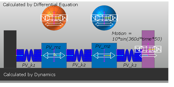
Figure 4.142 Differential equation model and verification model using dynamics

Differential equation_1 (Using explicit form)

The user can define a differential equation in an explicit form.

The equation using explicit form is following:

\(\left\{ \begin{aligned} & {{{\dot{q}}}_{1}}=\left( {{F}_{1}}-{{k}_{1}}{{q}_{3}}-{{k}_{2}}{{q}_{3}}+{{k}_{2}}{{q}_{4}} \right)/{{m}_{1}} \\ & {{{\dot{q}}}_{2}}=\left( {{F}_{2}}+{{k}_{3}}\delta +{{k}_{2}}{{q}_{3}}-{{k}_{2}}{{q}_{4}}-{{k}_{3}}{{q}_{4}} \right)/{{m}_{2}} \\ & {{{\dot{q}}}_{3}}={{q}_{1}} \\ & {{{\dot{q}}}_{4}}={{q}_{2}} \\ \end{aligned} \right.\)

Set the PV, VE, DE and Expression like as following:

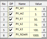
Figure 4.143 Set PV

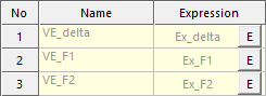
Figure 4.144 Set VE

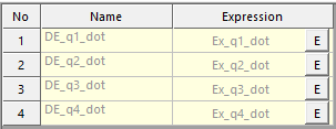
Figure 4.145 Set DE

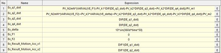
Figure 4.146 Set Expression

Differential equation_2 (Using implicit form)

The user can define a differential equation in an implicit form.

The equation using implicit form is following:

\(\left\{ \begin{aligned} & 0=\left( {{F}_{1}}-{{k}_{1}}{{q}_{3}}-{{k}_{2}}{{q}_{3}}+{{k}_{2}}{{q}_{4}} \right)/{{m}_{1}}-{{{\dot{q}}}_{1}} \\ & 0=\left( {{F}_{2}}+{{k}_{3}}\delta +{{k}_{2}}{{q}_{3}}-{{k}_{2}}{{q}_{4}}-{{k}_{3}}{{q}_{4}} \right)/{{m}_{2}}-{{{\dot{q}}}_{2}} \\ & 0={{q}_{1}}-{{{\dot{q}}}_{3}} \\ & 0={{q}_{2}}-{{{\dot{q}}}_{4}} \\ \end{aligned} \right.\)

Set the PV, VE, DE and Expression like as following:

Figure 4.147 Set PV

Figure 4.148 Set VE

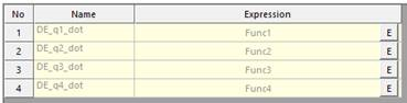
Figure 4.149 Set DE

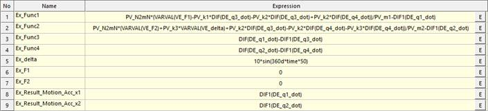
Figure 4.150 Set Expression

Results of differential equation

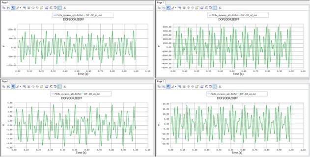
Figure 4.151 Comparison of differential equation results and dynamic analysis results