7.2.1.2. Interpolation
7.2.1.2.1. Definition of Interpolation Analysis
Interpolation helps you perform one-dimensional interpolation of the values in a curve to create an evenly spaced sampling of the curve values.
Linear
Use the first order Lagrange’s formula. The equations of linear interpolation are defined as,
If \(x_{k-1} \leq x_i < x_k (k=1,...,N)\),
\(y_i=\frac{x_i-x_k}{x_{k-1}-x_k} \times y_{k-1} + \frac{x_i-x_{k-1}}{x_k-x_{k-1}} \times y_k\)
Here \((x_0,y_0),(x_1,y_1),...,(x_{N-1},y_{N-1})\) are N points in curve data, \(x_i\) is the point at which to interpolate and is defined by interpolation region and the number of interpolated value, \(y_i\) is the interpolated value.
Polynomial
Through any two points there is a unique line. Through any three points, a unique quadratic. The interpolating polynomial of degree N-1 through the N points \(y_0=f(x_0),y_1=f(x_1),...,y_{N-1}=f(x_{N-1})\) is given explicitly by Lagrange’s classical formula,
There are N terms, each a polynomial of degree N-1 and each constructed to be zero at all of the \(x_i\) except one, at which it is constructed to be \(y_i\). A using algorithm (for constructing the same, unique, interpolating polynomial) is Neville’s algorithm.
\(y_i=P(x_i)\)
Here \((x_0,y_0),(x_1,y_1),...,(x_{N-1},y_{N-1})\) are N points in curve data, \(x_i\) is the point at which to interpolate and is defined by interpolation region and the number of interpolated value, \(y_i\) is the interpolated value.
2-order Polynomial makes Polynomial function using first 3 points in turn. The equations of 2-order polynomial interpolation are defined as,
If \(x_0 \leq x_i < x_2\),
\[\begin{flalign} y_i=P(x_i)=\frac{(x_i-x_1)(x_i-x_2)}{(x_0-x_1)(x_0-x_2)} \times y_0 +\frac{(x_i-x_0)(x_i-x_2)}{(x_1-x_0)(x_1-x_2)} \times y_1 +\frac{(x_i-x_0)(x_i-x_1)}{(x_2-x_0)(x_2-x_1)} \times y_2 \end{flalign}\]If \(x_{k-1} \leq x_i < x_k (k=3,...,N)\),
\begin{flalign} y_i=P(x_i) &=\frac{(x_i-x_{k-1})(x_i-x_k)}{(x_{k-2}-x_{k-1})(x_1-x_k)} \times y_{k-2} +\frac{(x_i-x_{k-2})(x_i-x_k)}{(x_{k-1}-x_{k-2})(x_{k-1}-x_k)} \times y_{k-1} \\ &+\frac{(x_i-x_{k-2})(x_i-x_{k-1})}{(x_k-x_{k-2})(x_k-x_{k-1})} \times y_k \end{flalign}3-order Polynomial makes Polynomial function using first 4 points in turn. The equations of 3-order polynomial interpolation are defined as,
If \(x_0 \leq x_i < x_2 < x_3\),
\begin{flalign} y_i=P(x_i) &=\frac{(x_i-x_1)(x_i-x_2)(x_i-x_3}{(x_0-x_1)(x_0-x_2)(x_0-x_3)} \times y_0 +\frac{(x_i-x_0)(x_i-x_2)(x_i-x_3)}{(x_1-x_0)(x_1-x_2)(x_1-x_3)} \times y_1 \\ &+\frac{(x_i-x_0)(x_i-x_1)(x_i-x_3)}{(x_2-x_0)(x_2-x_1)(x_2-x_3)} \times y_2 +\frac{(x_i-x_0)(x_i-x_1)(x_i-x_2)}{(x_3-x_0)(x_3-x_1}(x_3-x_2) \times y_3 \end{flalign}If \(x_{k-1} \leq x_i < x_k (k=4,...,N)\),
\begin{flalign} y_i=P(x_i) &=\frac{(x_i-x_{k-2})(x_i-x_{k-1})(x_i-x_k)}{(x_{k-3}-x_{k-2})(x_{k-3}-x_{k-1})(x_{k-3}-x_k)} \times y_{k-3} \\ &+\frac{(x_i-x_{k-3})(x_i-x_{k-1})(x_i-x_k)}{(x_{k-2}-x_{k-3})(x_{k-2}-x_{k-1})(x_{k-2}-x_k)} \times y_{k-2} \\ &+\frac{(x_i-x_{k-3})(x_i-x_{k-2})(x_i-x_k)}{(x_{k-1}-x_{k-3})(x_{k-1}-x_{k-2})(x_{k-1}-x_k)} \times y_{k-1} \\ &+\frac{(x_i-x_{k-3})(x_i-x_{k-2})(x_i-x_{k-1})}{(x_k-x_{k-3})(x_k-x_{k-2})(x_k-x_{k-1})} \times y_k \end{flalign}
Akima
The Akima interpolation is similar to the Hermite interpolation. Derivatives at nodes are calculated in the Akima interpolation, but derivatives at nodes are prescribed in the Hermite interpolation.
Polynomial
Let \(P_{01}(x)\) be an interpolation function at x ( \(x_0 \leq x \leq x_1\))
\(P_{01}(x)=f_0H_0(x)+f_0'K_0(x)+f_1H_1(x)+f_1'K_1(x), x_0 < x < x_1\)
- where,
- \(H_0=\frac{2}{h^3}(x-x_0+\frac{h}{2})(x-x_1)^2\)\(H_1=-\frac{2}{h^3}(x-x_0)^2(x-x_1-\frac{h}{2})\)\(K_0=\frac{1}{h^2}(x-x_0)(x-x_1)^2\)\(K_1=\frac{1}{h^2}(x-x_0)^2(x-x_1)\)\(h=x_1-x_0\)\(f_i'=\frac{|s_{i+1}-s_{i+1}| \times s_i + |s_i-s_{i-1}| \times s_{i+1}}{|s_{i+2}-s_{i+1}|+|s_i-s_{i-1}|}\)\(s_k=\frac{f_k-f_{k-1}}{x_k-x_{k-1}}\)
Initial and End points condition
The calculations of \(f_0', f_1', f_{n-1}'\), and \(f_n'\) using Eq.( ) are impossible since \(f_{-1}\) and \(f_{-2}\) are needed to calculate \(f_0'\), \(f_{-1}'\) is needed to calculate \(f_1'\), \(f_{n-1}'\) and \(f_{n+1}\) is needed to calculate \(f_{n-1}'\) and \(f_{n+1}\) and \(f_{n+2}\) are needed to calculate \(f_n'\).
Let an interpolation function f(x) be expressed as
\(f(x)=ax_2+bx+c\)
for points \(x_0\), \(x_1\), \(x_2\) and
\(\begin{matrix} ax_0^2+bx_0+c=f_0 \\ ax_1^2+bx_1+c=f_1 \\ ax_2^2+bx_2+c=f_2 \end{matrix}\) or \(\left[ \begin{matrix} x_0^2 & x_0 & 1 \\ x_1^2 & x_1 & 1 \\ x_2^2 & x_2 & 1 \end{matrix} \right] \left[ \begin{matrix} a \\ b \\ c \end{matrix} \right] = \left[ \begin{matrix} f_0 \\ f_1 \\ f_2 \end{matrix} \right]\)
By solving the above equation a, b, and c can be obtained. Derivation of Eq.( ) with respect to x gives \(f_0'\) and \(f_1'\) as
\(f_0'(x_0)=2ax_0+b\)
\(f_1'(x_1)=2ax_1+b\)
CSpline(Cubic Spline)
The cubic spline interpolation is to get an interpolation formula that is smooth in the first derivative, and continuous in the second derivative, both within an interval and at its boundaries. Given a tabulated function \(y_i=y(x_i), i=0,...,N-1\), focus attention on particular interval, between \(x_i\) and \(x_{i+1}\). The cubic spline interpolation in that interval gives the interpolation formula
\(y=Ay_i+By_{i+1}+Cy_i''+Dy_{i+1}''\)
- where,
- \(A \equiv \frac{x_{i+1}-x}{x_{i+1}-x_i}\)\(B \equiv 1-A=\frac{x_-x_{i+1}}{x_{i+1}-x_i}\)\(C \equiv \frac{1}{6}(A^3-A)(x_{i+1}-x_i)^2\)\(D \equiv \frac{1}{6}(B^3-B)(x_{i+1}-x_i)^2\)
The key idea of a cubic spline is to require the continuity between two intervals and to use it to get equations for the second derivatives \(y_i''\). For \(y_i''\) the following equations are obtained.
These are N-2 linear equations in the N unknowns \(y_i'', i=0,...,N-1\). For a unique solution, two further conditions are needed. For computing \(y_0''\) and \(y_N''\), initial and end conditions are used. The equation for points \(x_0\), \(x_1\) and \(x_2\) are expressed as
\(y=ax^2+bx+c\)
\(\begin{matrix} ax_0^2+bx_0+c=y_0 \\ ax_1^2+bx_1+c=y_1 \\ ax_2^2+bx_2+c=y_2 \end{matrix}\) or \(\left[ \begin{matrix} x_0^2 & x_0 & 1 \\ x_1^2 & x_1 & 1 \\ x_2^2 & x_2 & 1 \end{matrix} \right] \left[ \begin{matrix} a \\ b \\ c \end{matrix} \right] = \left[ \begin{matrix} y_0 \\ y_1 \\ y_2 \end{matrix} \right]\)
By solving the above equation a, b, and c can be obtained.
\(y_0''=2a\)
As same, \(y_{N-1}''\) is obtained by end condition.
7.2.1.2.2. Property
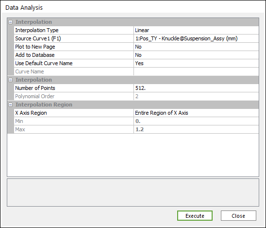
Figure 7.53 Data Analysis dialog box [Interpolation]
Interpolation
Interpolation Type: Selects a type of Interpolation.
Linear
Polynomial
Akima Spline
Cubic Spline
Source Curve: Selects a curve.
Plot to New Page: If the user wants to draw to new page, select Yes. If the user wants to draw to current page, select No. (The default option is No.)
Add to Database: If the user wants to add a desired result to the database, select Yes. (The default option is No.)
Use Default Curve Name: If you want to use the default curve name like “ADD(Acc_TM-Body1(mm/s^2), Vel_TM-Body1(mm/s))”, select Yes. If not, the Chart use the Curve Name.
Curve Name: If Use Default Curve Name is No, Chart use this for a name.
Number of Points: The default is 512. The user must enter a positive integer. If the user is preparing the curve for an FFT operation, RecurDyn/Plot recommends that the number of points be an even power of two (for example, 256, 512, 1024, and so on).
Polynomial Order: Sets the order of polynomial function. If the user selects Polynomial of Operation Type, this is activated.
Interpolation Region
X Axis Region
Entire Region of X Axis
Specified Region of X Axis: Set up Min and Max.
Min: Minimum X value.
Max: Maximum Y value.