7.2.1.6.2. Tutorial for Campbell Diagram

7.2.1.6.2.1. Step 1 Creating the Data for the Campbell Diagram

In the example model folder under the RecurDyn’s installation directory, open Gear_Model.rdyn. This model contains bevel gears, a helical gear and a worm gear. It was implemented using the GeoContact entity. The gear assembly is a dynamic model of a rotational machine system and requires the order tracking analysis. This model contains many possible joints and motions. This tutorial includes only those processes necessary to produce the Campbell diagram.

Example Model) <Install Dir>\Help\Examples\Campbell

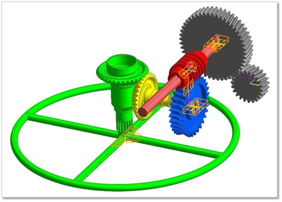
Figure 7.61 Gear model

Creating the Expression

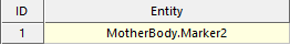
RevJoint2 of Subsystem1 contains the motion information and two reference markers: MotherBody.Marker2 and G1_Z27.Marker1. The user uses these markers to produce an expression that can extract the necessary data.

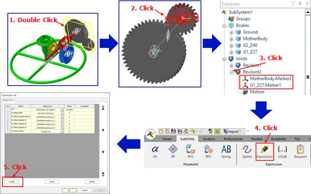
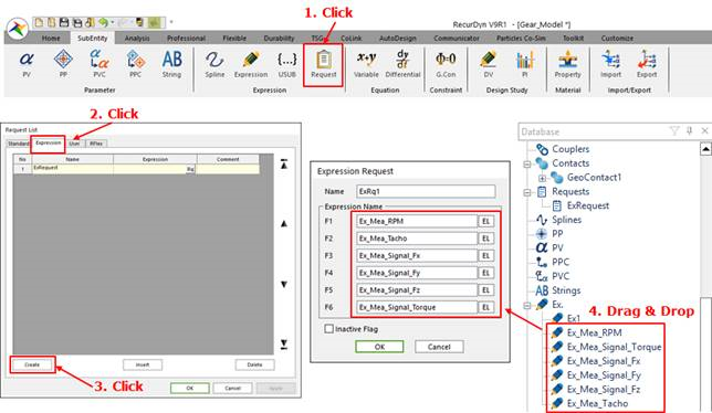
After performing the steps outlined in the preceding figure, the Expression List dialog box appears. This dialog box also includes the Expression dialog to create an expression. First, let’s produce an expression that extracts the RPMs.

• Producing the RPM Expression

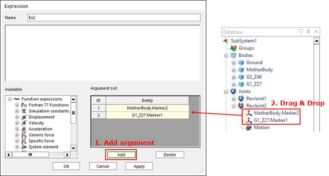
  In the Name field for the expression, enter Ex_Mea_RPM. Then, drag two markers from the Database window and drop them in Argument List.

  

  Expression	60*WZ(1,2,2)/(2*pi)
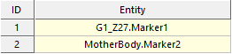
  Argument List

  This expression multiplies the speed caused by the WZ function acting on the two markers by 60 and divides it by 2π to convert it into RPM. For more information about the WZ function, refer to the How to use Velocity Functions.

• Producing the Tacho Expression

  Repeat the procedure for producing an RPM expression to create an expression that includes the two markers as arguments. Then, in the Name field for the expression, enter Ex_Mea_Tacho. Finally, enter the following information:

  Expression	sin(AZ(1,2))
  Argument List

  This function enters the two markers into a sine function to produce the sine wave signal for each rotation. For more details on the AZ function, refer to the How to use Displacement Functions.

• Producing the Signal Fx Expression

  Create an expression named Ex_Mea_Signal_Fx. Then, drag MotherBody.Marker2 from the Database pane and drop it in the Argument List. Finally, enter the following information.

  Expression	JOINT(RevJoint2,0,2,1)
  Argument List

  This function extracts the reaction force of the joint by measuring the X-axis load of RevJoint2. In addition, the reference coordinate is MotherBody.Marker2. For more information about the Joint function, refer to the How to use Joint Functions.

• Producing the Signal Fy Expression

  Create an expression named Ex_Mea_Signal_Fy. Input the same argument as for the Signal Fx expression, but enter JOINT(RevJoint2,0,3,1) for the expression. The user can also copy Ex_Mea_Signal_Fx, which was produced in the previous step, from the Database window and modify it.

  Expression	JOINT(RevJoint2,0,3,1)
  Argument List

• Producing the Signal Fz Expression

  Create an expression named Ex_Mea_Signal_Fz. Input the same argument as for the Signal Fx expression, but enter JOINT(RevJoint2,0,4,1) for the expression.

  Expression	JOINT(RevJoint2,0,4,1)
  Argument List

• Producing the Torque for the Signal Fz Expression

  Create an expression and named Ex_Mea_Signal_Torque. Input the same argument as for the Signal Fx expression, but enter JOINT(RevJoint2,0,8,1) for the expression.

  Expression	JOINT(RevJoint2,0,8,1)
  Argument List

To produce the Campbell diagram, you need the following data: RPM or tacho data and signal data. For this tutorial, the user can input any load, acceleration, speed, and displacement data as the signal data. This sample extracts the RPM and tacho data as well as the reaction forces acting on the joint.

Creating the Request

To display the output of the expression, the user must register a request. In the Subentity tab, click the Request icon to produce an expression request. Then, drag the expressions created from the Database window and drop them in the Expression Request dialog box. Finally, click OK.

Executing the Simulation

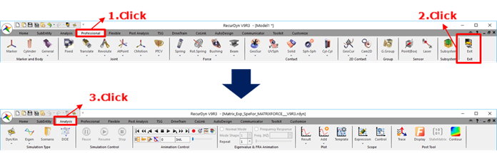
After the user has completed all of the preceding steps, exit the Subsystem mode. In the Professional tab, click Exit to switch to Model Edit mode. Click the Analysis tab.

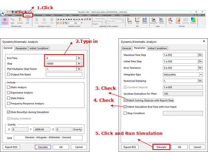
In the Analysis tab, click the Dyn/Kin icon to open the Dynamic/Kinematic Analysis dialog box. Enter information in End Time and Step. In the Parameter tab of the Dynamic/Kinematic Analysis dialog box, select Match Solving Stepsize with Report Step and Match Simulation End Time with User Input. Then, click Simulate.

Click the Plot icon to open the Plot window, and then ensure that the results appear.

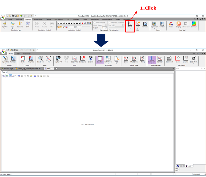
7.2.1.6.2.2. Step 2 Opening the Campbell Diagram Dialog Window

In the Tool tab of the Analysis group, click the Campbell Diagram icon to open the Campbell dialog box.

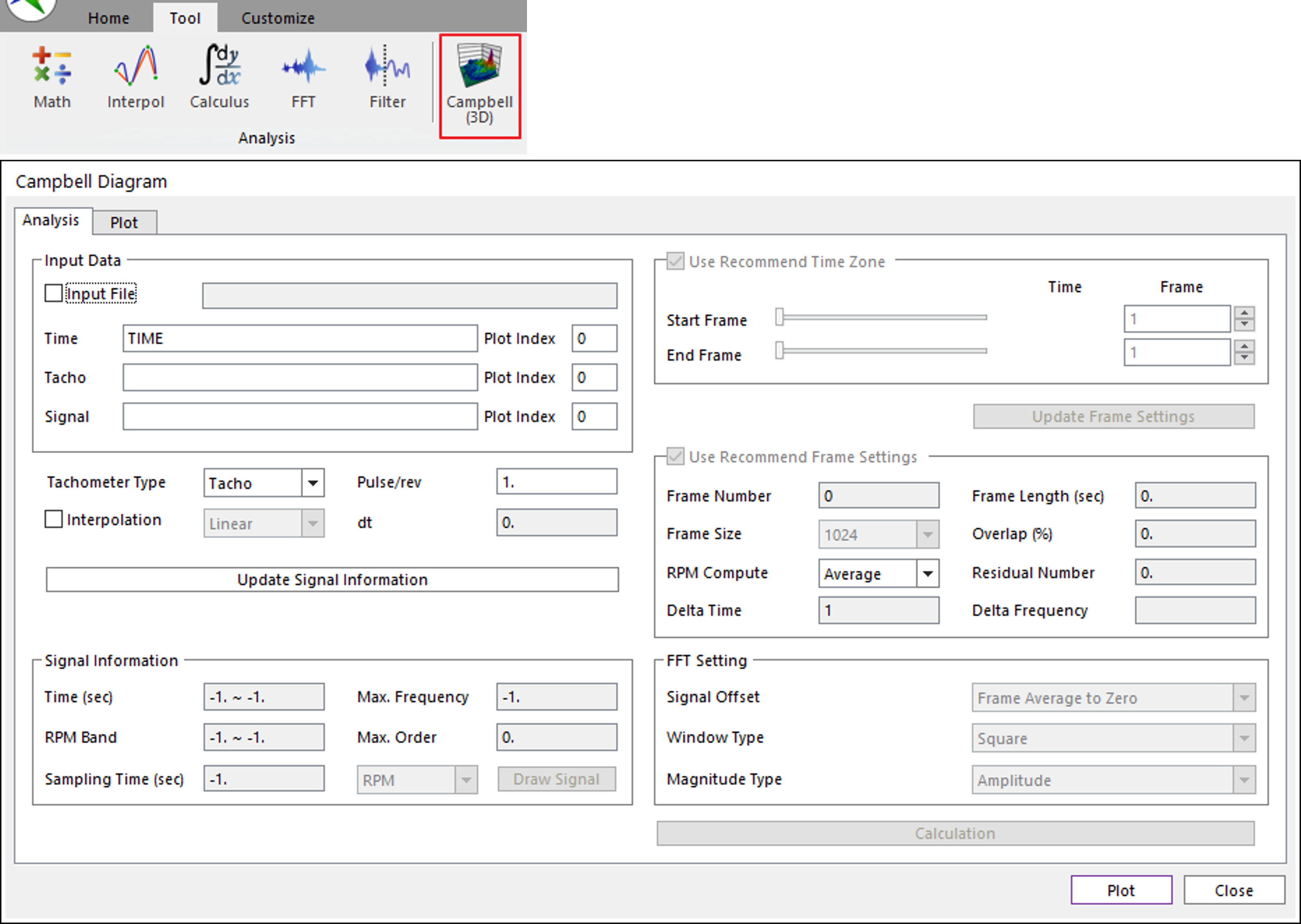
Note) The menus are shaded until data is entered.

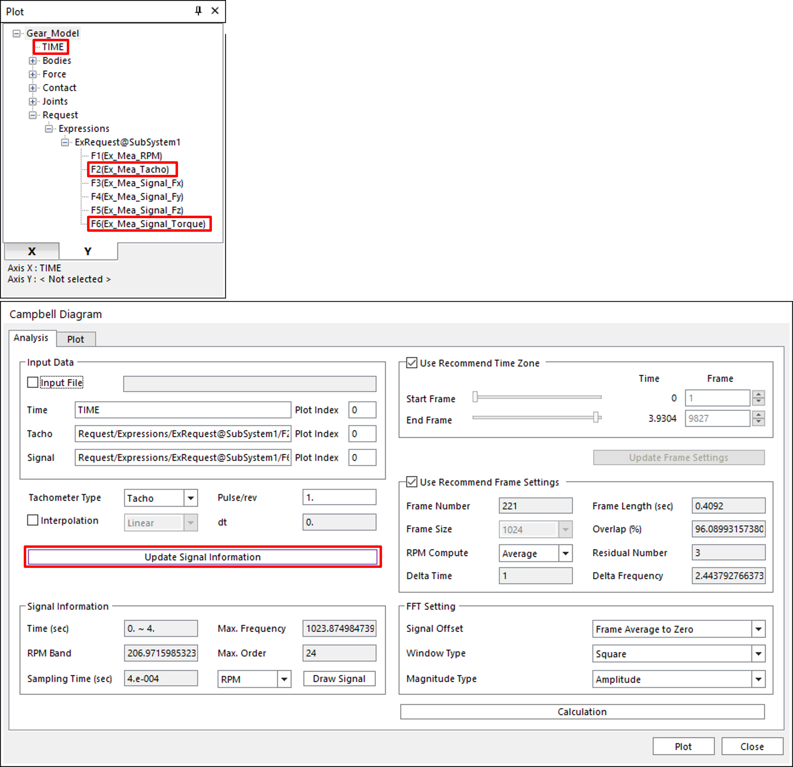
7.2.1.6.2.3. Step 3 Inserting Data into the Dialog Window

The data necessary to produce the Campbell diagram should appear in the Plot database window. If the RPM and signal data extracted from the test are in text files, then the user can drag and drop the text files into the Plot database window to register the data. This sample uses data from the analyzed Gear_Model. If you skipped the modeling tutorial and began this chapter from Plotting the Campbell Diagram section, then the user can drag and drop the Gear_Model.rplt file from the sample folder to the Plot database window to use as analysis results. The user can drag data from the Plot database window and drop it into the Campbell dialog box to enter it. If the user clicks Apply when the user has entered all of the data, all of the menus become activated and the Default Settings are selected.

• Pulse/rev or RPM Multiplier: After the user enters the tacho signal or RPM data, the final RPM is multiplied by the Pulse/rev or RPM Multiplier. The default value is ‘1.’ This function is used when the RPM of the entered signal is a multiple of the actual system RPM or when one cycle of the tacho signal is a multiple of the actual cycle.

  

• Interpolation: When the report step size is not uniform, the Interpolation is necessary. There are two interpolation types, Linear type and Spline type. The user check on the interpolation option, select the interpolation type and insert desired step size and the interpolated signal data is used for Campbell diagram.

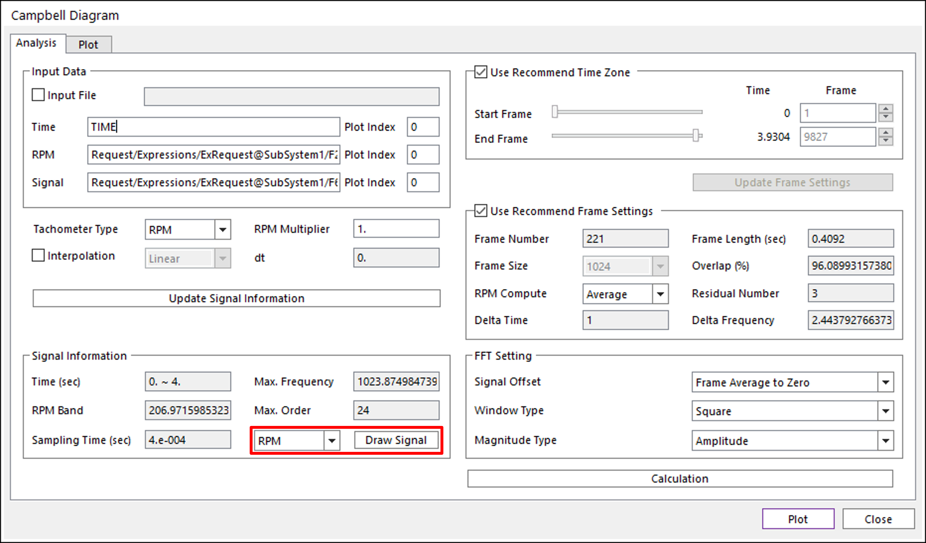
Note

If the Input type is changed from Tacho to RPM, the title displayed on the dialog, which is Pulse/rev is converted to RPM Multiplier, as shown in the figure.

7.2.1.6.2.4. Step 4 Draw Data

The Data Draw function, which can draw input data on the plot window directly. With this function, the user can review the total signal and the RPM data.

• Tacho: Draw the Time-Tacho data on the Plot Window.

• RPM: Draw the Time-RPM data on the Plot Window.

• dRPM: Draw the Time-dRPM data on the Plot Window, which differentiates the RPM data and is a function of time.

• Signal: Draw the Time-Signal data on the Plot Window.

• Signal FFT: Draw the signal data converted by the Fast Fourier Transform (FFT) algorithm on the Plot Window.

Note

Settings for Signal FFT Plot

• Data: Spline interpolation

• Signal Offset Method: Signal average to zero

• Window: Square

• Magnitude Type: Amplitude

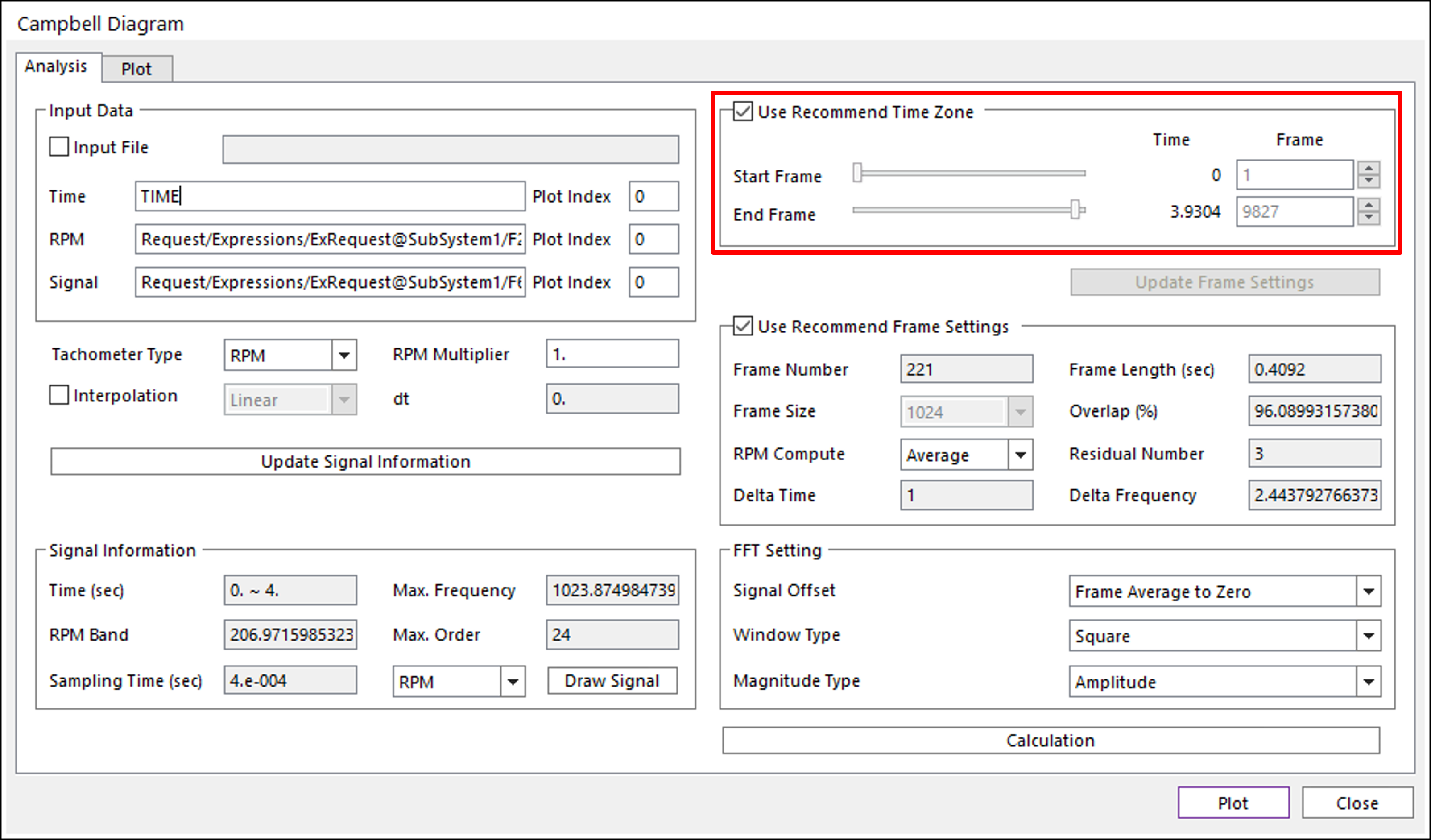
7.2.1.6.2.5. Step 5 Setting the Time Zone

The time zone defines the actual data frame used to draw the Campbell diagram when using only a portion of the entire analysis time.

• Use Recommend Time Zone: The Use Recommend Time Zone option automatically selects the zone for which linearity is guaranteed for the RPM data increase rate. If the system calculates the time differential values of the RPMs from the beginning to the end of the data and locates an increase or decrease above a certain value, then the zone of variance is excluded. If no zones of variance are found, then the system uses all of the data. The user can deselect Use Recommend Time Zone to select another time zone.

  

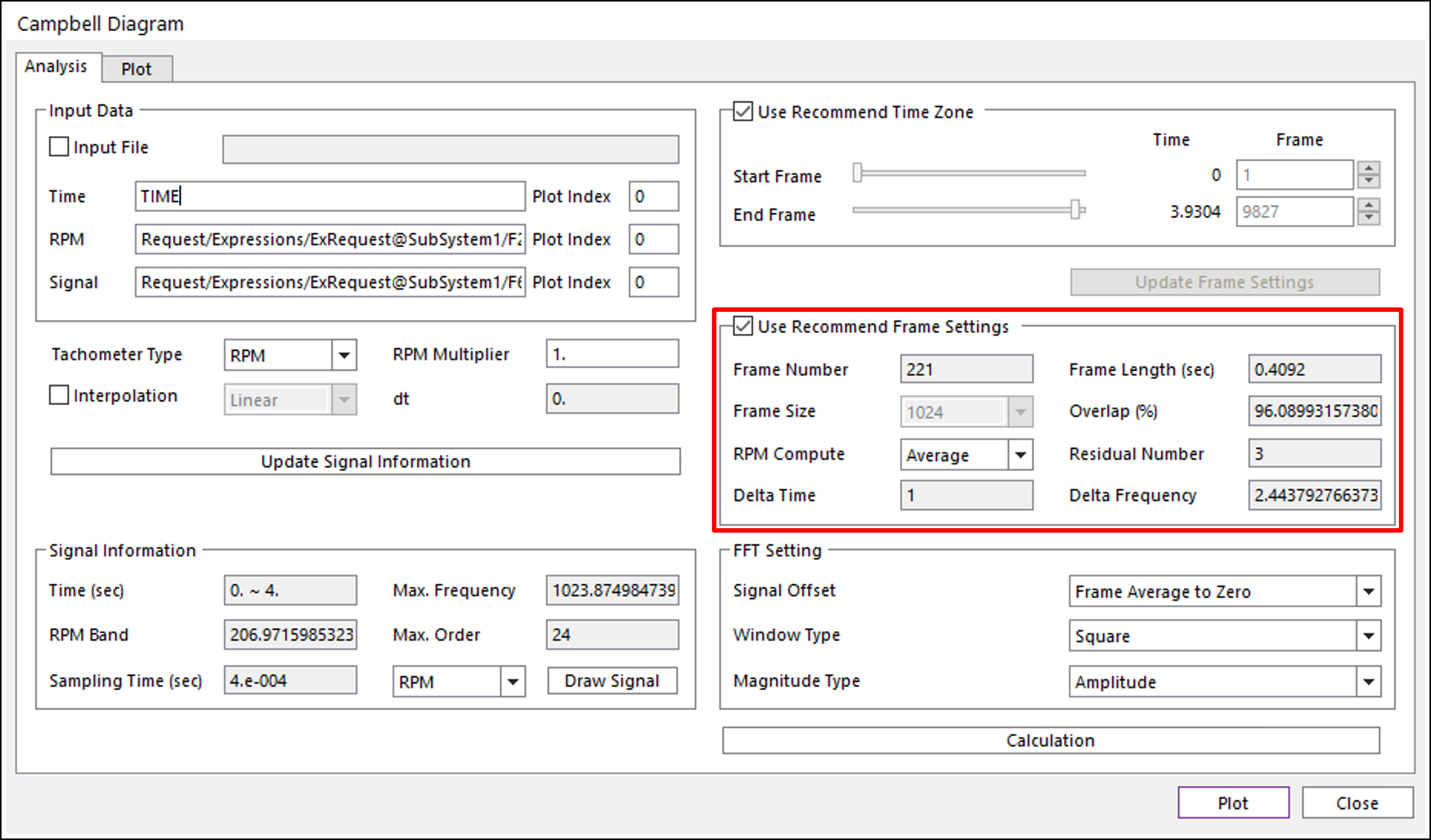
7.2.1.6.2.6. Step 6 Configuring the Frame Settings

The frame settings specify the size and number of frames to use in the STFT.

• Use Recommend Frame Settings: This option automatically selects the frame size based on the signal information. The system then locates and enters the minimum residual data count for the frame count, which is equivalent to 1/4 count of the frame size. This is determined based on the resolution and half as much frame size is produced as the frequency data. Wherever possible, the count for the X and Y data is also halved. If Use Recommend Settings are turned off, the user can change the desired setting.

• Delta Time: The Delta time setting allows to use the partial data among the extracted data rather than all of the data. The user can use this option when having a very long time period, but the response frequency is low.

• Frame Number: Specifies the frame count.

• Frame Size: Specifies the data count for each frame.

• Overlap(%): Specifies the percentage of overlapping data between neighboring frames.

  Note

  The input value must be between 0 and 100. Otherwise, when the user clicks Plot, an error message is displayed.

• RPM Compute: Calculates the representative RPMs for each frame using the average or min/max values.

• Frame Length: Specifies the time length of each frame.

• Residual Number: Specifies the number of data after a decimal point in the remaining data value.

  

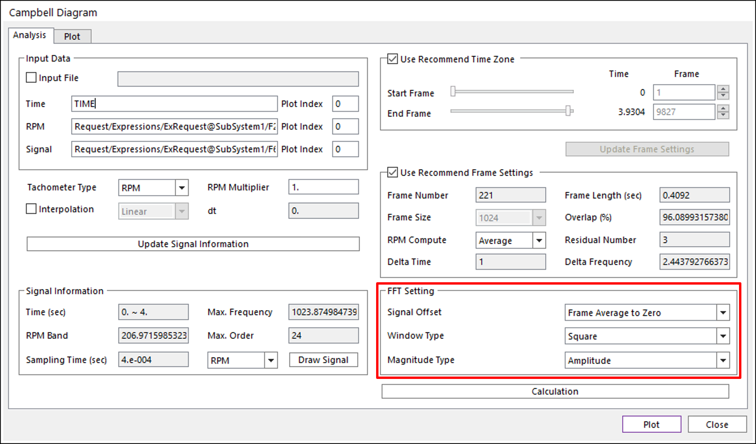
7.2.1.6.2.7. Step 7 Configuring the FFT Settings

The FFT settings determine how to conduct the FFT for each frame.

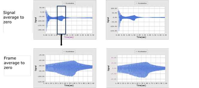
• Signal Offset: The signal offset method setting configures the offset for the signal frequency response to time. This function adjusts the frequency using the 0 set. This prevents problems that occur during overall tendency analysis when the low-frequency signal produces too large a value for the 0 frequency.

  

  • Signal average to zero: Subtracts the average value of the entire signal data from the signal data and uses the remaining value to offset the signal data.

  • Frame average to zero: Subtracts the average value of the frame from the frame data and uses the remaining value to offset the signal data when it contains the low-frequency signal.

  

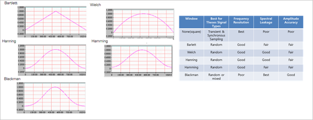
• Window Type: Since the signal format for the FFT signal handling cannot begin from 0 and end in 0, the user can use the Window function to adjust the signal format. RecurDyn includes the following Window functions.

  

• Magnitude Type: The magnitude of the resulting value calculated through the FFT can be expressed as an amplitude, power spectrum or power spectrum density. The user can use the following formulas to calculate these values.

  • Amplitude: Mean square of the real number and imaginary number.

    \(X(k)=\frac{1}{N} \left| \sum _{n=1}^{N} f_ne^{-i\omega n} \right|\)

  • Power Spectrum: Square spike

    \(PS(k)=(X(k))^2=\left(\frac{1}{N} \sum _{n=1}^{N} f_ne^{-i\omega n} \right)^2\)

  • Power Spectrum Density: This is a magnitude, so calculate it as though the energy of time data and energy of frequency data have the same physical quantity when the signal is speed. (For general PSD, df is not multiplied, but it is multiplied to express the area of each frequency in the mechanical field.)

    \(PSD(k)=df \cdot dt \cdot N \cdot \left( \frac{1}{N} \sum _{n=1}^{N} f_ne^{-i\omega n} \right) ^2\)

7.2.1.6.2.8. Step 8 Configuring the Plot Settings

The plot settings configure the processes used to draw the signal-processed results in Campbell Diagram.

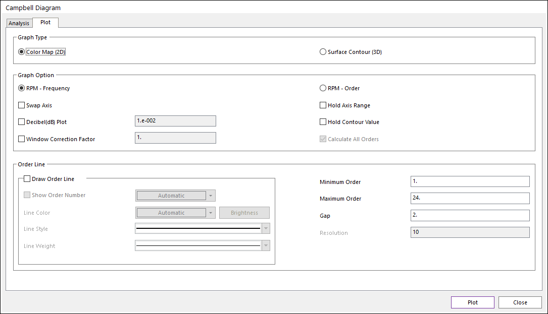
• Order Line: Specifies the frequency line that the RPMs show and allows a line to be drawn for the RPM value.

  • Frequency(Ω) = N*Ω/60 (N:Order, Ω:RPM)

  • A to B Gap C: A is the beginning value of N and B is the ending value. The gap is the interval of increasing N.

• Draw Order Line: Specifies whether to draw the order line.

7.2.1.6.2.9. Step 9 Drawing and Modifying the Campbell Diagram

After the user configures all of the settings, click Plot to draw the Campbell diagram.

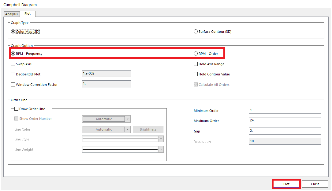
• RPM-Frequency: Shows the magnitude value to the RPMs against frequency graph

• RPM-Order: Expresses the frequency using order by converting the RPMs against frequency graph. The following is the formula for the conversion.

  • N = Frequency*60/ Ω (N:Order, Ω:RPM)